
I2AO Part 8c: Spacecraft
Back to the Index of I2AO (Introduction to Astronomy Online)
| Previous |
PART 8c: SPACECRAFT by Ian Kemp
Feel free to take an adventure through all these entries, or take the links from the table to learn about specific spacecraft. Ian Kemp has selected some of the more interesting examples of lunar and planetary robotic explorers, satellites, rovers, and space telescopes to discuss here.
| 1 Sputnik | 2 Vanguard | 3 Explorer 1 |
| 4 Ariel 1 | 5 Syncom | 6 Luna 2 |
| 7 Luna 3 | 8 The Rangers | 9 Luna 9 |
| 10 Surveyor | 11 Luna 16 | 12 Venera 7 |
| 13 Venera 13 and 14 | 14 Mars 2 and 3 | 15 Rosetta |
| 16 NEAR Shoemaker | 17 A broken promise | 18 Hayabusa2 |
| 19 OSIRIS-Rex | 20 Lunokhod 1 | 21 Sojourner |
| 22 Spirit and Opportunity | 23 Cháng’é | 24 Curiosity |
| 25 Huygens | 26 Himawari | 27 LRO |
| 28 Parker Solar Probe | 29 MESSENGER | 30 New Horizons |
| 31 IKAROS | 32 Galileo | 33 MOM - Mangalyaan |
| 34 Cassini | 35 Voyager 2 | 36 Juno |
| 37 GALEX | 38 Kepler | 39 WMAP |
| 40 Spitzer | 41 LISA Pathfinder | 42 Chandra |
| 43 HST |
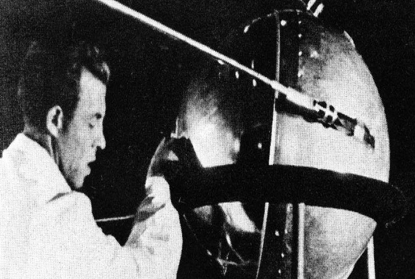
1: PS, aka Sputnik
On 4 October 1957, a Russian R-7 ICBM rocket fired the first artificial satellite into space: “PS”. After the control crew confirmed that it was actually in orbit (by picking up its radio transmissions during its 90-minute orbit) they renamed it “Sputnik 1” and announced to the world that the USSR had placed the first satellite into Earth orbit.
The Russian representatives to a conference on space observation of Earth, being held in New York, were just as surprised as the Americans and reps from other nations, but they found it hard to hide their smiles. The Americans had assumed that they were technological world leaders, and the successful launch of Sputnik 1 was a huge blow to the national ego, which demanded a response. Therefore, it could be said that Sputnik 1 started the ‘space race’ and has a direct line of connection to the manned Moon landings.
The original plan was to launch a multi-purpose scientific probe, (which would later be launched as Sputnik 3), but a decision was made to send up a much simpler object to reduce risk. Sputnik 1 was a polished aluminium sphere about 60 cm in diameter, containing two radio transmitters and a set of silver-zinc batteries. The sole function of the device was to broadcast a ‘beep’ using four antennae stuck to the outside of the sphere. The Russians made well-known the frequencies Sputnik used to transmit - 20 and 40 MHz, and also the visibility timetable, to make sure that any backyard enthusiast could tune in with a simple radio set. The craft totalled 85 kg and actually contained a nitrogen atmosphere - it was not internally in vacuum.
It beeped away for about three weeks, after which the batteries were ‘flat’. After 96 days, its orbit had decayed to the point where it fell into the atmosphere and burned up.
Figure 1.1 Sputnik
Image Credit: NASA / ASIF A. SIDDIQI
2: Kaputnik, aka Vanguard
(Please note, this will be the only mention of a craft that was built but did not fly in space.)
After the successes of Sputnik 1 and Sputnik 2, pressure was put on the US space industry to launch a satellite to respond to the Soviet success. In a deliberate contrast to the secretive Soviet approach, the press was invited to come along and watch the launch of the US response, Vanguard, on 6 December 1957. The policy of openness backfired badly when the Viking rocket carrying the Vanguard probe managed an altitude of just one metre, before crashing to the ground in a sea of flames. Not only was Vanguard tiny compared to Sputnik (just 1.5 kg and about the size of a grapefruit), but it seemed to mock the US achievements by surviving the rocket failure and beeping away from its position on the ground not far from the launch pad.
The mission was lampooned in the press as “Kaputnik”, “StayPutNik” “Dudnik” and “Flopnik”.
Needless to say, the political embarrassment caused by the Sputnik program and the poor initial US response spurred on the US technical teams to much greater efforts.
Video: View the non-launch video here.
Figure 2.1 Vanguard
Image Credit: US naval research laboratory

3: Explorer 1 - JPL begins its run!
After the ignominy of Vanguard, the US President gave the Army Ballistic Missile Agency and the Jet Propulsion Lab (JPL) three months to get a satellite into space.
JPL designed and built Explorer 1 - a scientific mission, containing sensors to measure cosmic rays and micrometeorites, and radio the data back to Earth. Explorer 1 was a long cylindrical craft, about two metres long and 16 cm in diameter. It was successfully launched on top of a Jupiter C ICBM launcher on 31 January 1958 and began sending back data. It travelled in a highly elliptical orbit varying in height from 354 km (a bit lower than the orbit of today’s International Space Station) to 2500 km. Thus, it was able to measure radiation and micrometeorites over a wide range of heights, informing scientists about these potential hazards to future space flight.
Anomalies in the data led the mission scientist, James van Allen, to conclude that the spacecraft was passing through bands of dense radiation shaped by Earth’s magnetic field - and thus the Van Allen radiation belts were discovered by the US’s first space mission.
Figure 3.1 Explorer 1: Explorer 1 is the whole of the cylinder down to the fins near the upper left - the science and engineering payload fill roughly the top half of the spacecraft.
Image Credit: NASA

4: Who’s your daddy? – Ariel 1
On 26 April 1962, the UK became the third country to operate a satellite when Ariel 1 was launched using a US Thor-Delta rocket at Cape Canaveral. Responsibility for the spacecraft seems to depend a bit on who’s telling the tale, but the fact is that the UK Science Research Council (SRC) approached the newly-formed US National Aeronautics & Space Administration (NASA) with a proposal for a scientific mission to measure the effect of solar emissions on the Earth’s ionosphere. This was in response to the US offering to help other nations with space technology.
Ariel 1 was a joint effort with British scientists, funded by the SRC designing and supplying the science payload, and NASA’s Goddard Space Flight Center providing engineering and packaging it. The launch was provided by the US. The spacecraft was about 60 cm in diameter and 20 cm high, and weighed 62 kg. The instruments to study different aspects of solar radiation, and the Earth’s ionosphere, were powered from NiCd batteries charged using a set of solar panels. The machine had a tape recorder on board, capable of storing 100 minutes worth of data (one orbit’s worth), which would then be downlinked when it was in a suitable position (if you don’t know what a tape recorder is, ask your grandparents!). Ariel 1 flew in an eccentric orbit, with the altitude varying from 397 km to 1200 km.
It operated for a bit over two months, at which point the solar panels were damaged by radiation from a US high altitude nuclear bomb test. It was actually switched on again and successfully sent data for three months in 1964. It finally fell to destruction in Earth’s atmosphere in 1976.
Figure 4.1 Ariel 1: The photo shows a replica of Ariel 1, built at the Goddard Space Flight Center using spare parts and leftovers - it is located at the Steven F. Udvar-Hazy Center in Chantilly, VA.
Image Credit: Smithsonian Institute
5: Limited offer, slow moving stock, one for the price of three! - Syncom
I hope you all remember from my series on Moons (or of course you quite likely knew it already) - the orbital period of a satellite increases with altitude. This feature of Newtonian gravity produced some confusion during spacewalks by the early US astronauts. The problems happened during docking practice on Gemini 4 (1965). The pilot used the attitude thrusters to try and 'catch up' with the target spacecraft in the same orbit - and was quite surprised to find that he started falling back! (the tangential thrust had raised him into a higher orbit). It took some time to learn that to close up correctly they had to apply thrust angled up away from Earth so they would fall into a lower orbit and catch up with the target.
In the 1940s, famed author, Arthur C Clarke, realised that at a certain altitude a satellite would orbit with a period of exactly one day, so if placed in orbit above the equator it would appear to be stationary to people on Earth. This, he said, would be a great spot to put communications satellites. Fast forward to the early ’60s, and the first Geostationary satellite, Syncom 3, was launched on 19 August 1964. It was manoeuvred into geostationary orbit on 23 September and was then used, among other things, to transmit live TV coverage of the Tokyo Olympics to the US. In addition to this commercial use, radio signals from the probe were analysed by scientists to work out some of the properties of the Earth’s ionosphere - an important contribution to our ongoing understanding of issues to do with communications and spacecraft performance. Later, Syncom 3 was co-opted by the US military and used for communications to support the US war on Vietnam.
BUT! before Syncom 3, there was Syncom 2! This was basically the same design and was a pathfinder for Syncom 3. It was the first satellite put in geosynchronous orbit. This means it orbited once per day but, because it wasn’t over the equator, it continuously wobbled between the northern and southern hemispheres. Not good as a long-term comms satellite, but it proved the basic technology without going through the complex orbit adjustments needed to move it from its launch latitude to the equator.
The 71cm-diameter, 39cm-high cylindrical package contained fuel and a rocket motor and was covered with solar cells which charged a NiCd battery array. The payload was a fairly standard (for the early ’60s) radio repeater set. At the underside of the cylinder, you can see in the photo below, the attitude control jets which were used to align the object and you can also see the external antennae. The Syncom satellites were built by the Hughes Aircraft Corporation.
Now you may not realise this, but a geostationary (or geosynchronous) orbit is quite high - at 35,800 km above Earth’s surface, it is around one tenth of the way to the Moon. Syncoms 2 and 3 were launched using an upgraded version of the Thor-Delta rocket earlier used for Explorer 1 (a Delta rocket mounted on top of a Thor ICBM launcher). In case you were wondering, Syncom 1 was the same design and was launched, but had a comms failure after launch.
Figure 5.1 Syncom 2
Image Credit: NASA

6: Go somewhere where there’s cheese! Luna 2
The early history of missions to the Moon is a litany of launchpad explosions, failed upper stages and navigation gone wrong. Getting to the Moon is hard, and lessons were learned the expensive way.
The first spacecraft to actually reach the Moon was Luna 2 (Луна 2), launched 12 September 1959 - and when I say reach the Moon, I mean crash onto it. Don’t be fooled by the number “2” - the Russian practice at the time was to only name probes that actually went somewhere and got some results.
Unlike Sputnik 1, Luna was a scientific mission - it carried instruments to measure the ionosphere and the magnetic field - it provided new data on those of Earth and basically showed that the Moon has no magnetic field. It also carried some explosives, a small payload of sodium and some small USSR flags. The intention of the first two was to produce a cloud of sodium on impact, so that Earth observatories could confirm the landing and the location. The purpose of the latter was maybe to try and impress any Lunians who might come across the wreckage.
Due to the increasingly chilly Cold War with the USA, the Russians tipped off British scientist Bernard Lovell as to the radio frequencies being used for telemetry, and the calculated time and position of impact. It was measurements by Lovell that persuaded the US that they had been once again scooped to a major space milestone. The stinger was the doppler shift in the radio signals, which proved they were coming from a fast-moving spacecraft.
Luna 2 produced no photos or video, but it did send back lots of data from its instruments, which were printed out on teletype paper - allegedly 14 km of it. Science was different in them days, kids!
By the way, before Luna 2 was Luna 1, officially recorded as a ‘flyby’ - which is to say, it missed.
Figure 6.1 Luna 2
Image Credit: NASA

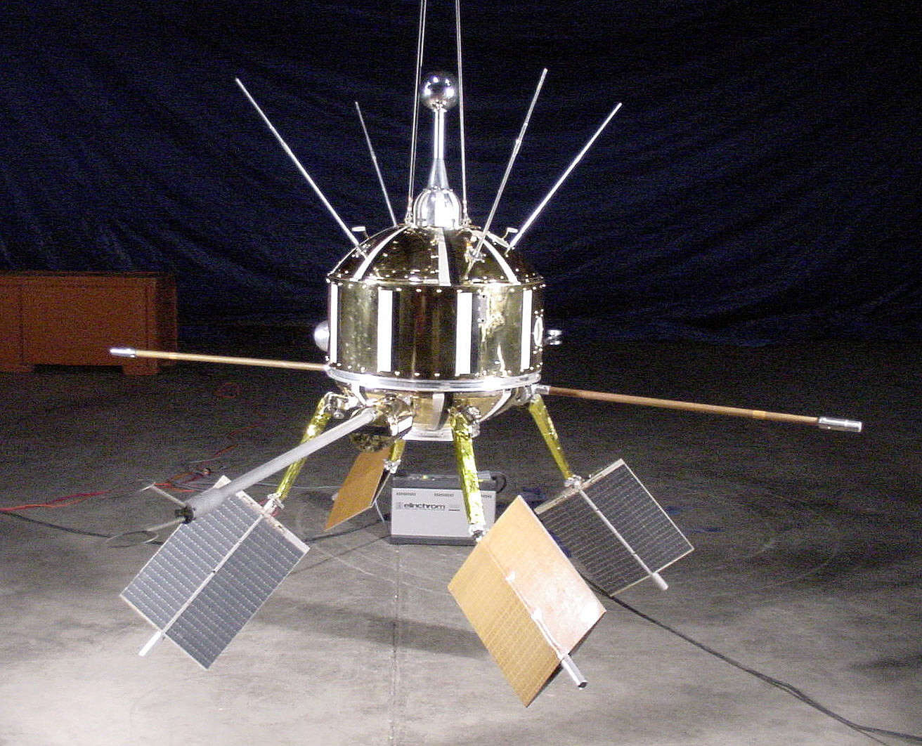
7: The far side – Luna 3
As politicians and scientists in the USA slowly turned green with envy, the USSR launched on 4 October 1959 the first mission to return images of the far side of the Moon.
Luna 3 was quite a sophisticated spacecraft - with propulsion and attitude control: photocells detected the Sun and the lit face of the Moon so that the propulsion system could turn the craft to face the right way. As usual, it carried instruments to measure the ionosphere and cosmic rays - but its main payload was a camera with two lenses (200 mm and 500 mm) and an on-board photo-processing and scanning system. There were no digital cameras in those days! A roll of 40 35mm negatives was exposed, then chemically developed and fixed, after which a scanning light source was used to convert the negatives into a stream of data which could be transmitted by radio back to Earth. This whole automated sequence was triggered when the photocells detected that the camera lenses were pointing towards the sunlit face of the far side of the Moon.
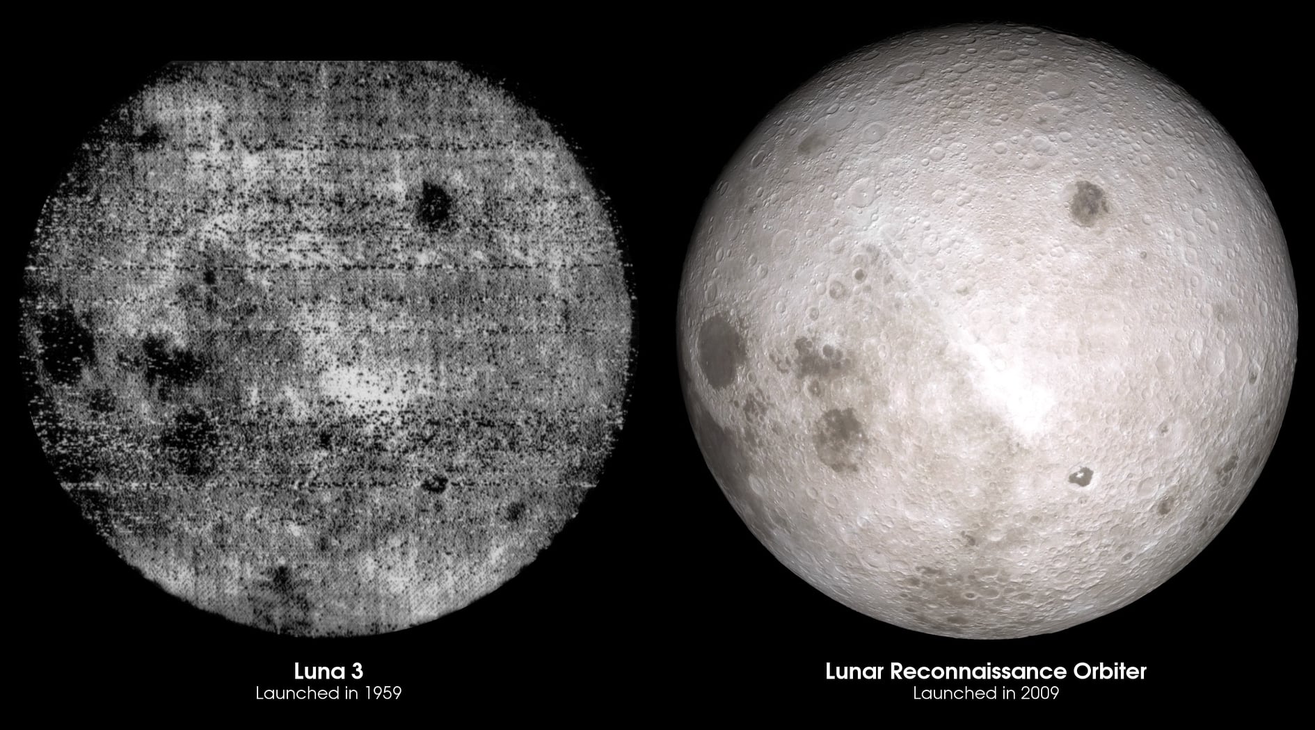
This was all quite impressive technology and the reward was humankind’s first view of the far side - and the scientifically important finding that the far side lacked the large ‘mare’ (dark patches which we now know to be lava lakes), which are so obvious on the near side of the Moon. The far side was mostly light-coloured highlands. So, now, people could begin to speculate on the history and formation of the Moon, having in hand some concrete evidence of its unusual structure, added to the knowledge from Luna 2 that it has no magnetic field.
Luna 3 did one shot around the far side then returned to Earth. Eventually it burned up in the atmosphere, though no-one is exactly sure when, because its telemetry had long since failed and, in those days, we didn’t have the sophisticated radar tracking available today to spot such a small object. It was only about one metre high and one metre across.
Figure 7.1 Replica of Luna 3 in the Memorial Museum of Astronautics
Image Credit: Photo by “Armael”

Figure 7.2 Side by side comparison of the first ever photo of the far side (from Luna 3) with a modern photo from the Lunar Reconnaissance Orbiter
Image Credit: NASA
8: A win's a win! – the Rangers
The US had multiple frustrations in its attempts to land a probe on the Moon. The Pioneer series from 1958 to 1960 and, then, the first few Ranger probes produced no results.
The first US probe to actually contact the Moon was Ranger 4, launched in April 1962. It had modest goals - simply a video camera payload to transmit close-up pictures of the surface as it zeroed in and crashed on the Moon. Unfortunately, Ranger 4 impacted on the far side of the Moon, and no data were received.
The next near thing was Ranger 6 (launched 2 Feb 1964) which hit the Moon, on the near side, but due to an electrical malfunction its cameras had activated shortly after lift-off and the batteries were well and truly flat by the time it was close enough to return useful data.
At last, on 31 July 1964, a winner was launched - Ranger 7 fulfilled its mission of crashing into the Moon, and returning photos during its approach. The scientific value of the mission was modest - but, at the time, the photos contributed to our understanding of the nature of the Lunar surface. The US ‘Man on the Moon’ program had been announced three years earlier, but it was still not known whether the Moon’s surface was rocky or a sea of soft dust - important information in the design of the Apollo landers. Ranger 4 was designed and built at JPL; it totalled 381 kg, of which 172 kg was the actual payload. It had a steerable dish antenna to send video data back to Earth - part of this is visible behind the solar panels in the photo.
Figure 8.1 Ranger 6
Image Credit: NASA

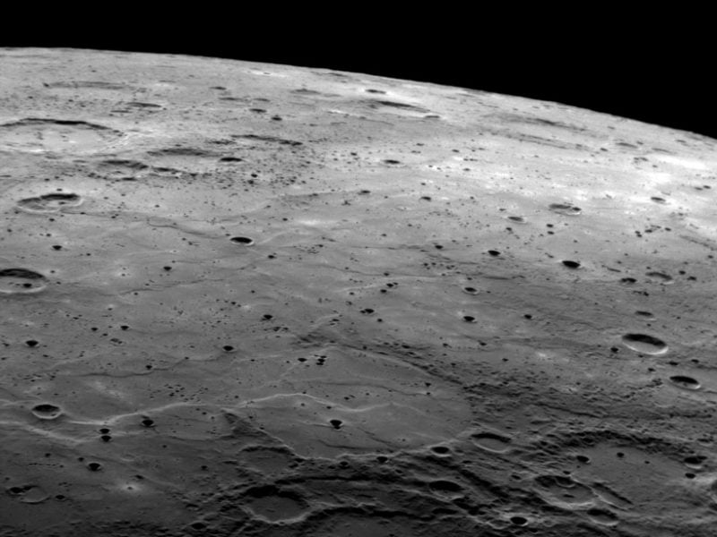
Figure 8.2 The Moon: The last complete photo received from Ranger 7 before it hit the Moon - taken at an altitude of 14 km, 2.3 seconds before impact, with a resolution of just half-a-metre. The area shown is about 2.8 km across.
Image Credit: NASA

9: Touchdown! – Luna 9
On 31 January 1966, Russian engineers launched the 12th in a series of attempts to make a ‘soft’ landing on the Moon. The mission succeeded when, on 3 February, Luna 9 touched down and began sending back landscape photos from the surface of the Moon.
The spacecraft consisted of a descent module and a landing module, together weighing over 1.5 tonnes. It was designed by GSMZ imeni Lavochkina, who were to become the USSR and Russian equivalent to the JPL in the USA. After blasting off from Baikonur Cosmodrome in Kazakhstan, on top of a Molniya-M + Blok L launch system, the machine was on course for the Moon.
The spacecraft used retro-rockets to shed speed during the descent and, when a height probe hit the surface, it released the landing module which, protected by airbags that inflated on the way down, bounced a few times before coming to rest on the surface of the Moon. The lander opened up four ‘petals’ tearing open the airbags and giving it positional stability, after which the camera system went into action and photographed a number of panoramas of the Lunar scenery.
In addition to the camera and telemetry, Luna 9 carried a gamma-ray spectrometer and a radiation detector, to collect more information on potential hazards to life and electronics in the space environment. The most important bit of scientific information from the mission was that the surface did not consist of soft dust, and it was solid enough to support a landing.
Either with or without the knowledge of the Russians, British scientists led by Bernard Lovell (whom you may remember from Luna 3) used the Jodrell Bank radio telescope to track the spacecraft and realised that the data transmissions used a fairly standard format. After the landing, they received the data, reconstructed the images, and sent them to the BBC, who published them for all the world to see.
Figure 9.1 Replica of the Luna 9 descent & lander assembly: Housed in La Musée de l'air et de l’espace, Paris
Image Credit: Photo by “Pline”
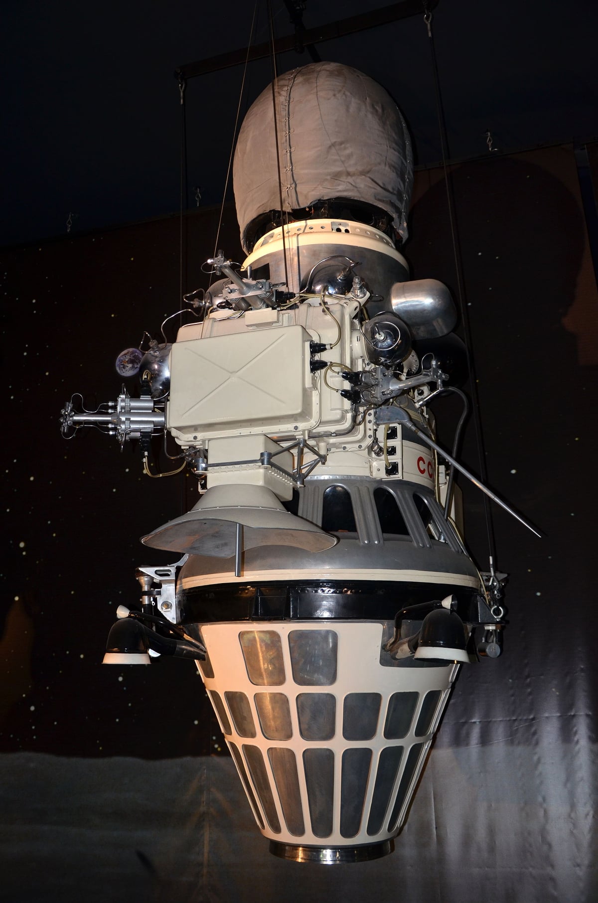
Figure 9.2 Luna 9 lander
Image Credit: S.P. Korolev RSC “Energia”

Figure 9.3 Image of the Moon’s surface from Luna 9
Image Credit: NASA

10: Surveyor
Surveyor 1 was the first US probe to ‘soft land’ on the Moon (i.e. survive the landing!). Like Luna 9, it used retro-rockets to slow its descent but, instead of using airbags, it just dropped the last few metres in the low Lunar gravitational field. Launched on the lucky day of May 30 1966, it plopped into place on the Moon on 2 June.
The integrated descender/lander weighed in at just under a tonne, and was built by Hughes Aircraft Corporation. The mission was, as usual, managed by JPL. Unlike the USSR approach, the lander used splayed legs with pads to land on the surface.
The spacecraft didn’t carry any scientific equipment apart from a video camera to collect images of the surface, but it had a number of sensors for its own control system (force, temperature, etc.) which, incidentally, provided some information about conditions on the Moon.
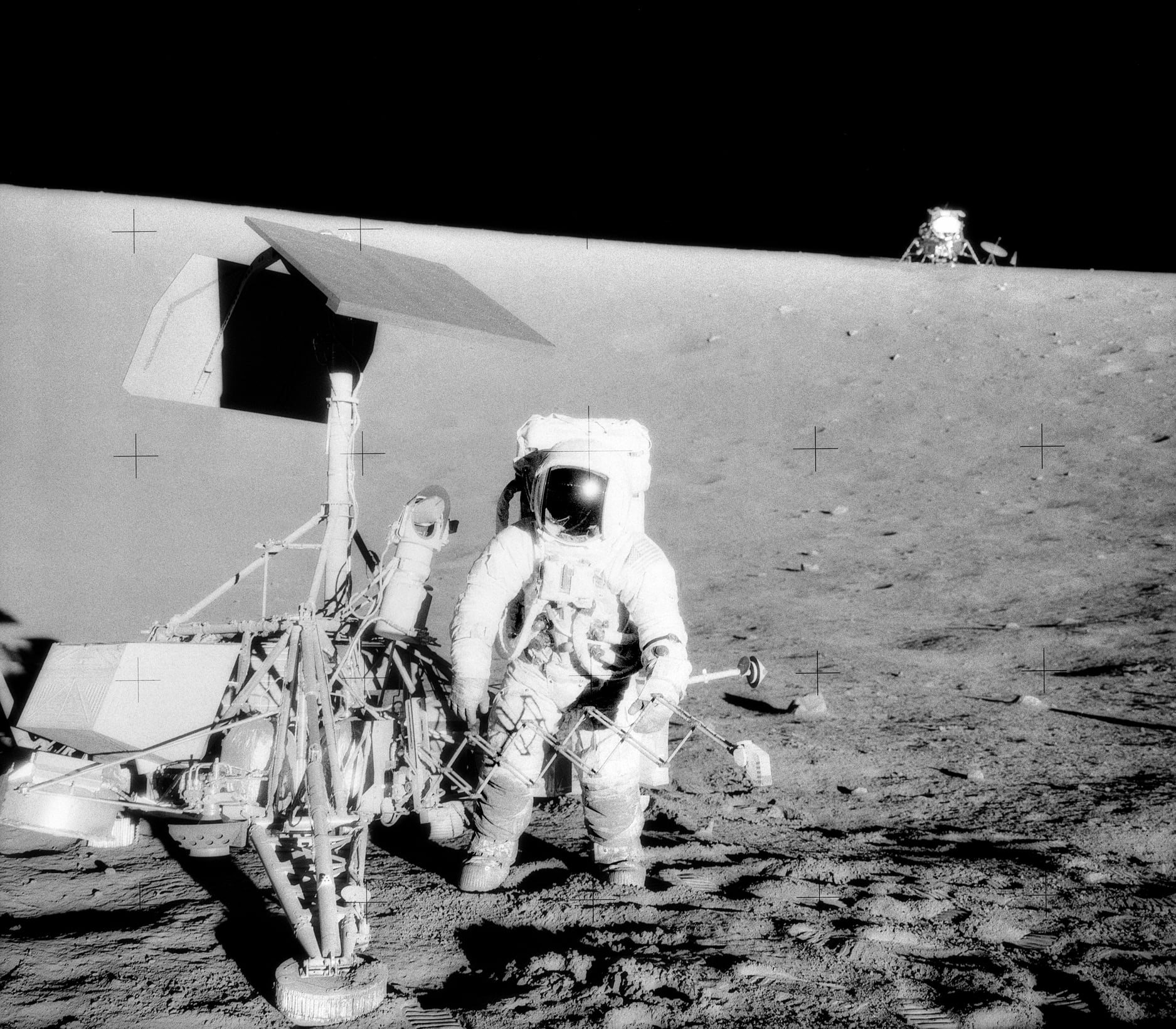
The photo shows Surveyor 3, which also completed a soft landing, shown actually on the Moon, photographed by the Apollo 12 astronauts who visited it. the Apollo 12 lunar module is visible in the background, and the second photo shows the size of Surveyor relative to astronaut Pete Conrad.
I still maintain it looks a bit like an accident in a junk shop, but most of the parts were functional. The two panels at the top are one solar panel and one planar radio antenna; sticking out to the right (half way up) is the video camera - the camera looks upwards onto a mirror which was angled around to allow photos in different directions. At lower right is a telescopic sampling arm for scraping up samples of the lunar soil - this was part of Surveyor 3 but was not installed on Surveyor 1.
Figure 10.1 Surveyor 3
Image Credit: NASA

Figure 10.2 Surveyor 3 and Pete Conrad
Image Credit: NASA
11: Moondust! Luna 16
One of the many scientific advances of the US Apollo program was the return of large amounts of ‘Moonrock’ to the Earth, where it could be analysed using sophisticated techniques and instruments in the best labs in the world. Moonrock from Apollo is still being analysed today, and revealing new information (for example the structure of water chemically combined into the rocks) with the help of newly-developed instruments that didn’t exist in the 1960s & 1970s.
But did you know that the USSR had its own collection of Moon samples? True! The Luna 16 spacecraft was launched on 12 September 1970 - shortly after Apollo 12 returned to Earth - and landed on the Moon on 24 September. The 2-tonne machine used retro rockets for most of its descent, and dropped in free-fall for about the last two metres, landing on its four stubby legs. Luna 16 landed on the near side - but in the dark, the first time this had been done. Shortly after landing, it unleashed its primary science payload - a drill set which angled down on to the surface and drilled a hole about 30 cm deep. The cuttings from the drill were dumped into a small collector and, about 24 days later, the upper stage lifted off from the Moon under its own rocket power.
The return pod eventually parachuted to Earth and landed in Kazakhstan where it was picked up by mission scientists. 100 grams of Moonrock for a fraction of the cost of the Apollo mission! The bottom part of the lunar lander stayed on the Moon, collecting data on radiation and temperature, and TV images, which were radioed to Earth.
This probe is one of my favourites because it began to show the greater potential of robotic missions, which would go on to dominate space exploration after the later Apollo missions were cancelled.
Figure 11.1 Luna 16: Now that’s what a proper steampunk spacecraft should look like! Luna 16 replica at the музее Космонавтики (Cosmonautics Museum), Moscow.
Image Credit: Photo by “Bembmv”
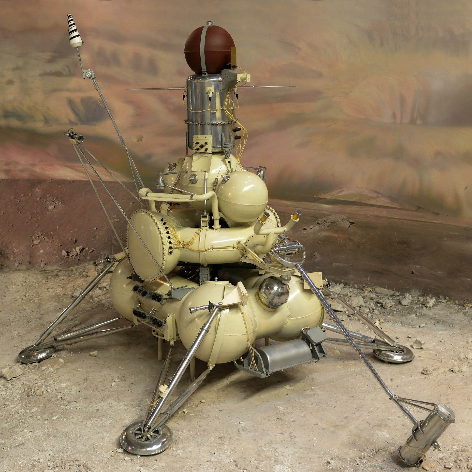
Figure 11.2 USSR postage stamp issued to commemorate Luna 16
Image Credit: Stanley Gibbons catalogue number 3886

12: Not in Kansas any more! Venera 7
On 15 December 1970, Venera 7 landed on Venus and thereby became the first Earth-built spacecraft to land on another planet in one piece. A number of earlier probes - flybys and attempted landings - had established that it was going to be a difficult environment for a spacecraft. Venera 4 had entered Venus’s atmosphere and shown that it was mostly carbon dioxide (with a bit of nitrogen), confirmed temperatures of up to 500 degrees C, and allowed an estimate of surface pressure of 100 Earth atmospheres.
Earlier landers, Venera 5 and Venera 6, entered the atmosphere but were crushed by the massive atmospheric pressure before they could reach the surface.
After these failures, the design was beefed up by placing the payload in a titanium shell intended to withstand 180 atmospheres. To compensate for the excess weight, engineers removed some of the telemetry from the upper stage of the launch vehicle. The lander retained its complete payload of instruments to measure internal and external temperatures, pressure, and the composition of the atmosphere. When it reached Venus, and the lander separated from the upper stage rocket, it was found that the channel switcher had failed, meaning that the craft could only send one channel of data, being the temperature channel it was stuck on. Pretty much as planned, Venera 7 descended, using a parachute, which survived until the craft was about 10 metres off the surface, at which point it free-fell and landed with a bang. At this point, it appeared to die and send no more data, but careful study of the mission recording tapes back on Earth sometime later showed that it had, in fact, transmitted 20 minutes of temperature data from the surface, in addition to the data sent during the descent. The signal had been very weak and engineers set about extracting the data from the random ‘noise’ on the tape.
The craft revealed that the surface temperature of Venus was around 470 degrees C and, from this, it was possible to calculate an atmospheric pressure of around 90 atmospheres. The hard landing showed that the planet had a rocky surface, at least at the part where Venera 7 came down! In 1972, a repeat expedition by Venera 8 was slightly more successful and returned more data including proof that the globe-encircling cloud layer stopped well above the surface - meaning that it would be feasible for future missions to take photos at the surface.
The information from Venera 7 & Venera 8 was used to help design future probes, including Venera 13, which sent back the first pictures of Venus’ surface, in 1982.
p.s. “Venera” is the Russian name for “Venus”.
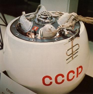
Figure 12.1 Development copy of Venera 7: The mission scientists believe that the reason the signal was so faint is that the spacecraft ended up lying on its side, with the body partly shielding the antenna. In the photo, it looks as if the antenna is along the body of the shell but, actually, it is held some distance above and away from the shell. Of course, with the terminal 10-m drop, its possible that the antenna was damaged.
Image Credit: NASA
13: Lab - clear for landing - Venera 13, 14
Venera 13 reached Venus on 1 March 1982. (The chart #1 in Australia on that day was “Tainted Love” by Soft Cell*, just to make you feel old!). Compared with the pioneering probes, Venera 13 was a veritable flying laboratory. It carried all the basic instruments: thermometer; barometer; accelerometer; etc., but also had some much more advanced equipment including a drill rig; two x-ray fluorescence spectrometers, one to measure the composition of the soil, the other the atmosphere; a mass spectrometer; a gas chromatograph; and a soil penetrometer to measure the strength of the soil. Given there was basically no hope of a sample-return mission to Venus in the foreseeable future, the Soviet scientists apparently opted to take the lab to the planet. It also had a colour TV camera and sent back some colour photos from the surface. The lander weighed in at just under a tonne and was 2.7 metres high.
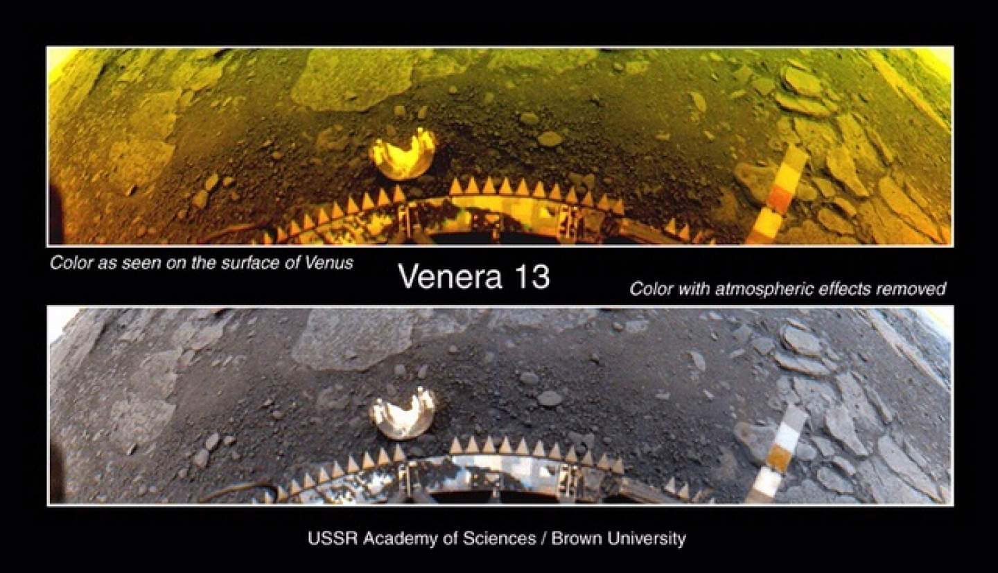
It was one of a pair - its twin, Venera 14, landed a few days later on 5 March 1982. Results from the two probes together provided a detailed chemical analysis of the atmosphere - and proved that it absorbed most of the ultraviolet light arriving from the Sun (so no sunburn on Venus!) Isotopic analysis of the gases in the atmosphere provided important data for models of the formation of the Solar System (adding to data from Earth and Mars). They also showed that the clouds were mainly sulphur containing (i.e. sulphur dioxide). The probes also made detailed measurements of the Venusian soil, and showed that it was similar to compacted ash, like volcanic tuff found on Earth. Most amazingly, Venera 13 sent back colour photos of the surface - see the photo below. The upper image is the raw colour photo - the colour of the rocks is dominated by the yellowish colour of sunlight filtered through Venus’s sulphur dioxide clouds. The lower image is a simulation of what the surface would look like in raw sunlight without the effect of the clouds.
All the science results were obtained and transmitted back in about two hours, after which the probe succumbed to the Venusian environment. This mission was, of course, after the end of Apollo and strengthened the case that robotic probes were the best approach to planetary exploration.
* The two guys who comprised “soft cell” were my neighbours in Leeds at the time.
Figure 13.1 Venera 13
Image Credit: NASA
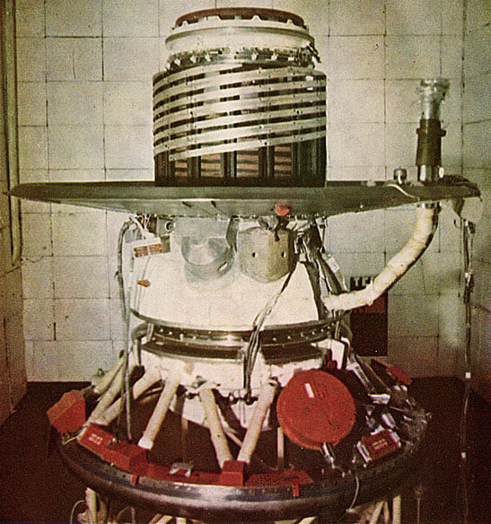
Figure 13.2 Venera 13 with labels
Image Credit: NASA
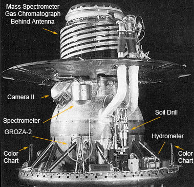
Figure 13.3 Raw and processed images from the surface of Venus
Image Credit: USSR Academy of Sciences/Brown University
14: The Red Planet – Mars 2 and 3
The Soviet Union scored another notable success in the ‘space race’ by landing the first spacecraft on Mars. A pair of twins, imaginatively named Mars 2 and Mars 3, were Launched on 19 May 1971 and 28 May 1971, respectively (Mars 1 had been sent two years earlier but lost communications before its approach to Mars). [The Australian #1 song at the time of both launches was appropriately enough “Spirit in the Sky” by Norman Greenbaum].
In each case, a two-stage Proton-K heavy lift rocket was launched from Baikonur, carrying the Blok-D 3rd stage and an orbiter/lander payload. The orbiter and lander were based on proven technology, and the lander was similar in design to Luna 9 which had successfully touched down on the Moon five years earlier. The 4MV orbiters sent back a bunch of atmospheric and geophysical data about the Red Planet. Unfortunately, it just happened that one of Mars’ occasional planet-wide dust storms was in progress at the time, so the orbiters sent back lots of photos of red dust swirling in the atmosphere.
In each case, the descent module had at its heart a 1.2m-diameter spherical capsule, attached to a vehicle able to use retro-rockets and parachutes to control the descent. The instrument capsules had TV cameras, temperature, pressure and wind speed probes, a mass spectrometer to analyse the atmosphere, and a soil scoop with instrumentation to analyse the surface materials and detect any signs of life (personally I have never understood why people have a fixation on the idea of “Life on Mars” - perhaps you can explain?). Most awesome of all, each lander had a little autonomous rover vehicle which could get around on skis, making measurements of surface hardness and density. Sadly, Mars 2 clapped out - the parachute did not deploy and the spacecraft crash-landed so the little ski rover didn’t see action that day! But Mars 2 retained the dubious honour of being the first Earth-built object to pollute the surface of Mars. Mars 3 did quite a bit better - it made it to the surface in one piece, and started returning data! Unfortunately, it died after 20 seconds so, once again, the ski-mobile didn’t get a run. Or maybe it did, and it’s just that the data never made it back? One day when someone visits the site of the landing, we might find out if the skiers ever skied.
Figure 14.1 Schematic of Mars 2 & 3 orbiter
Image Credit: NASA
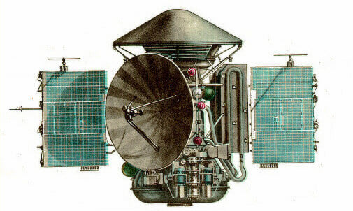
Figure 14.2 Photo of Mars 2 replica in the NPO Lavotchkin Memorial Museum of Cosmonautics
Image Credit: Public domain
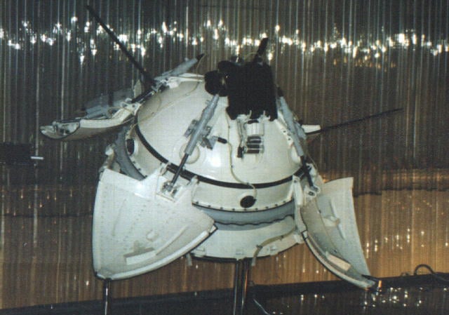
Figure 14.3 Skimobile
Image Credit: NASA

15: Comet Crunch - Rosetta
No spacecraft has landed on any planet apart from the ones we’ve already covered: Earth, Venus and Mars. Things have landed "in" Jupiter and Saturn (we will meet them later), but are they planetary landings? The moons of the outer Solar System are interesting places and I think more work and $$ should be put into exploring them.
We can now turn to some of the non-planets that Earth-made machines have visited.
Rosetta is a classic beauty in this series. Funded and built by the European Space Agency (ESA), it blasted off from the ESA launch site in Guiana on 2 March 2004, on top of an Ariane 5+ launch vehicle. Like many modern probes, Rosetta was scheduled to pass multiple science targets. Its primary mission was to get to the comet 67P/Churyumov–Gerasimenko, and on the way to visit two asteroids - 2867 Šteins and 21 Lutetia. The two discoverers of the target comet, Klim Churyumov and Svetlana Gerasimenko, were at the launch site in South America as VIPs when the craft was launched.
Another feature quite common with missions was the use of gravity assist. Rosetta passed Earth, then Mars, then Earth again to get a gravity assist to build up its velocity enough to match with the target comet. On the way, it collected some high-resolution photos of Mars, and collected photos and data from the two asteroids in the Main Asteroid Belt between Mars and Jupiter.
In August 2014, it rendezvoused with Comet 67P/Churyumov–Gerasimenko, and orbited the cometary nucleus. The 2.8m x 2m x 2.1m, three-tonne spacecraft carried a range of instruments with which to study the comet and, on 12 November 2014, it released its secret weapon ... the 100kg lander called Philae, which was equipped to carry out detailed chemical analysis of the comet. Unfortunately, Philae was a bit of a bust because it landed in a kind of crevice in the comet’s surface, where its solar panels were in shadows, and it quickly ran out of electrical power. The decision was made to take the main Rosetta craft down to a crash landing. After several months collecting data, it gently descended and became one with the comet on 29 September 2016. The mission returned a mountain of information on the composition of the comet, very useful for understanding conditions in the early Solar System.
Figure 15.1 Rosetta
Image Credit: ESA

Figure 15.2 Comet 67P/Churyumov–Gerasimenko
Image Credit: ESA

Figure 15.3 Churyumov and Gerasimenko at the launch site in Korou
Image Credit: ESA

16: Eros, NEAR Shoemaker
On 12 February 2001, the USA could at long last claim to have beaten the Russians to a landing on another body in the Solar System - when the spacecraft “Near Earth Asteroid Rendezvous” (“NEAR Shoemaker”) touched down on the surface of 433 Eros - a “Mars crossing” asteroid that approaches the Sun closer than the orbit of Mars for part of its 643-day year.
NEAR Shoemaker was designed by Johns Hopkins University Applied Physics Lab, and was launched by NASA on 17 Feb 1996. Its actual targets were changed due some problems at the gravity-assist encounter with Earth, but it passed close by asteroid 253 Mathilde in 1997 and eventually made it to its main objective, 433 Eros, on 14 Feb 2000. The 1.7m, 800kg spacecraft was carrying a battery of scientific instruments, including a multispectral camera, x-ray/gamma-ray spectrometer to measure the surface composition of the asteroid(s), near infrared spectrograph to make maps of variations in composition of the surface, a magnetometer to measure the magnetic field (if any), and help understand the internal structure of the asteroid, a laser rangefinder to accurately map the surface, and the ability to use the comms radio to map the gravity field (which can be used in conjunction with the rangefinder to look for variations in density).
The craft spent a year in orbit around Eros; mission scientists continually varied the orbit to enable measurements at different heights and directions. At the end of the mission, what to do with the spacecraft? I know! Let’s crash it into the asteroid! Decision taken, NEAR Shoemaker was directed down towards the surface, collecting and transmitting data as it went. To the staff’s surprise, when it impacted the surface, it just kept right on collecting data and sending it back! It finally gave up the ghost after sending back accurate close-range measurements of the surface composition for 16 days.
Figure 16.1 Artist’s impression of NEAR Shoemaker in flight
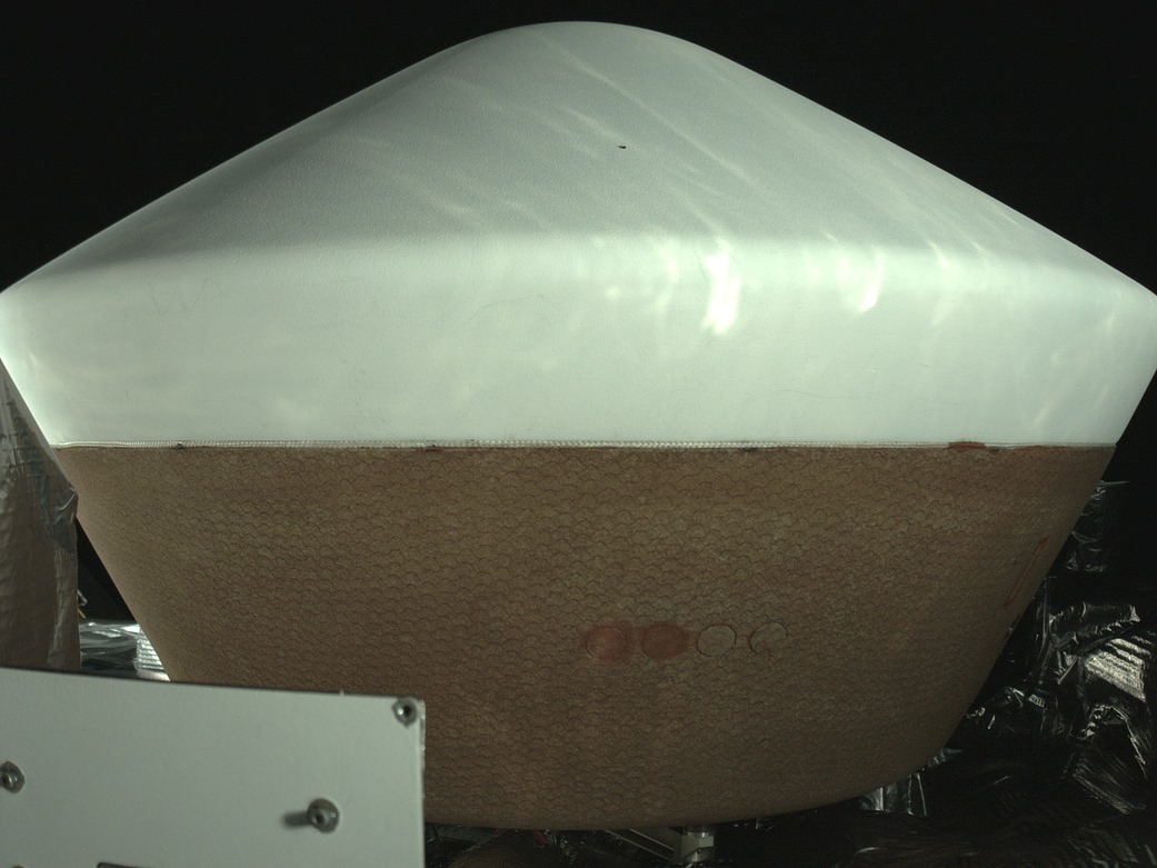
Image Credit: NASA

Figure 16.2 NEAR packed into the nose fairing on its Delta launch rocket
Image Credit: NASA
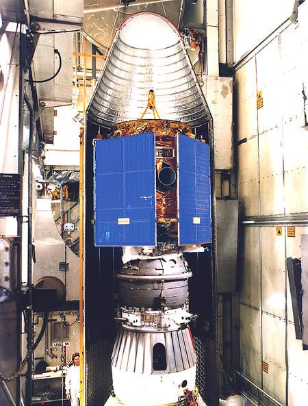
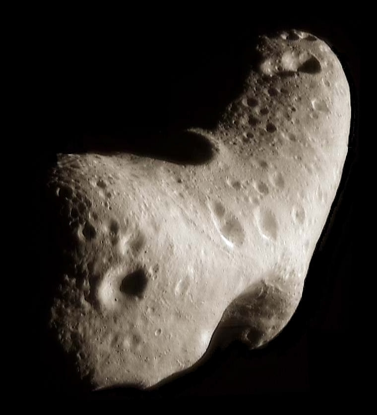
Figure 16.3 Image of 433 Eros
Image Credit: NASA
17: A broken promise
Here is a graphic prepared by Charles Apple, a US-based visual communicator who produces ‘in depth’ pages like this for a Washington State newspaper among lots of other good stuff! The broken promise is that it’s about a probe that has not yet been built - sorry about that, but a good read!
Figure 17.1 Capturing an Asteroid
Image Credit: Charles Apple

18: If one is good, two must be better! Hayabusa2
As we saw with Rosetta and Philae, if your exploration strategy consists of dropping a lander on a minor body, it might all be for nothing because comet nuclei and small asteroids can be irregularly shaped and sometimes be more like a loose jumble of rock and ice - a small lander might fall into a hole or be unable to ‘rove’ over a bouldery surface. So: how about taking a bunch of them to drop at likely looking places, spotted using the orbiter? And think of a propulsion method that means it can get around if it should get into trouble?
Meet はやぶさ2 = Hayabusa2 = Peregrine Falcon 2, a mission of the Japanese Space Agency (JAXA), to return samples from 162173 Ryugu - an irregularly shaped and bouldery near-Earth asteroid about one kilometre across. The mission was designed incorporating lessons from an earlier probe Hayabusa (which returned asteroid samples in 2010). The spacecraft was designed and built in Japan by NEC, incorporating a range of remote sensing equipment, and four landers, three of which were developed in Japan, and one in Germany (in collaboration with French scientists). On 3 December 2014, the mission blasted off from the Japanese Tanegashima Space Centre, using a Japanese H-IIA launcher (built by Mitsubishi Heavy Industries). It arrived at asteroid Ryugu in mid-2018 and began its work.
The three Japanese rovers were designed to hop around the surface using the movements of internal reaction masses (the same way that ‘Mexican Jumping Beans’ jump), and scope out suitable spots on the surface for the main vehicle to collect samples. The European rover carried a number of scientific instruments to collect data about the mineralogy and magnetic properties of the asteroid. Once the targeting rovers had done their jobs and identified ideal spots to collect samples, Hayabusa2 descended and collected samples. In two cases, it fired ‘bullets’ at the surface and collected the ejected dust. In the third case, it dropped some explosives onto the surface to blast out a small crater, then came in to collect pristine sub-surface material from the bottom of the crater.
The samples were put into canisters inside a ‘return capsule’ and, on 13 November 2019, the spacecraft fired up its ion engine to return to Earth. Sometime later this year (2020), it will get close enough to drop the return capsule and, all going to plan, the capsule will parachute to Earth at the Woomera rocket range in South Australia.
Figure 18.1 Asteroid Ryugu, photographed by Hayabusa2 in 2018
Image Credit: ISAS, JAXA, Hyabusa2 Team

Figure 18.2 Spacecraft ready for assembly to the launcher
Image Credit: ISAS, JAXA, Hyabusa2 Team
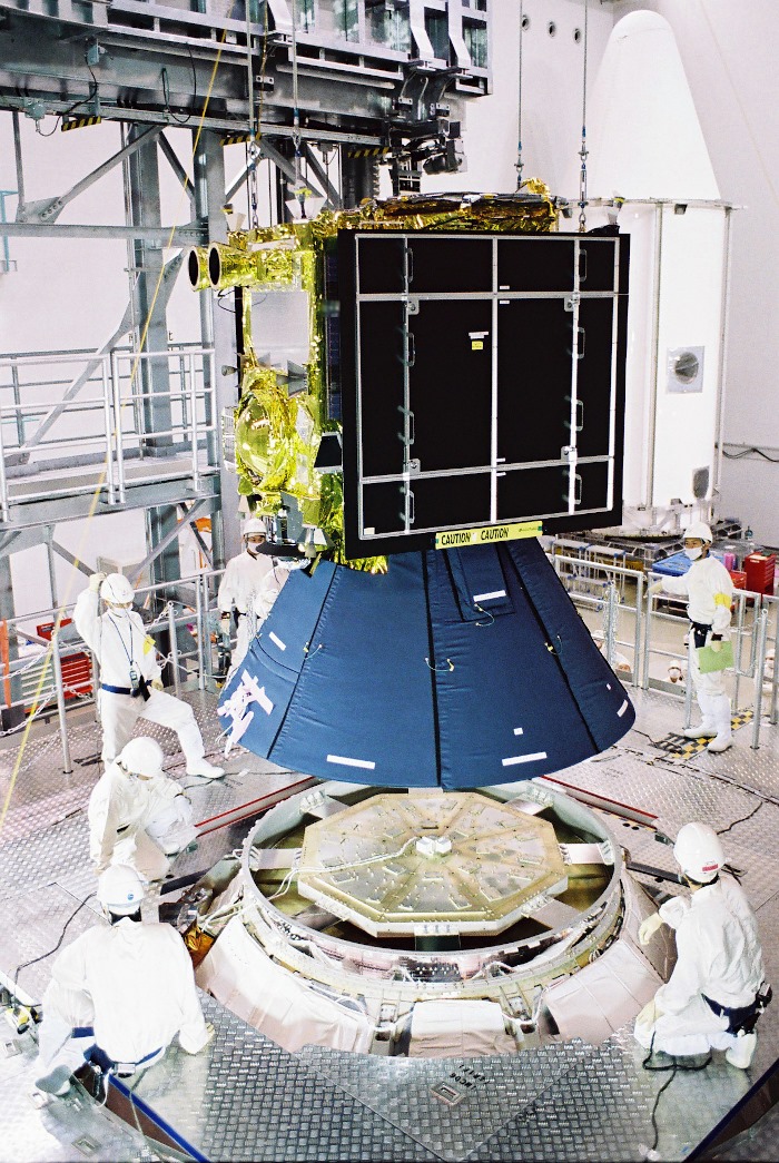
Figure 18.3 Sample return capsule
Image Credit: ISAS, JAXA, Hyabusa2 Team

19: Play it again Sam! OSIRIS-Rex
OSIRIS-Rex is NASA’s return-samples-from-an-asteroid mission. The US mission is less complex than the Japanese Hayabusa2, but has similar science goals and a similar target - a carbonaceous near-Earth asteroid. Like Hayabusa2, it is motivated by a desire to understand the early origins of the Solar System, and the origins of life, by studying naturally-occurring carbon-based molecules found on the asteroid. The difference is that the target, 101955 Bennu, is in an orbit that could well see it crash into Earth, precipitating a major catastrophe for Earth-based life. One of the science goals of OSIRIS-Rex is to get a lot more information on the mass, density, shape and reflectivity of the asteroid, so that we can more accurately model its orbit and understand the likelihood of it coming down upon us in its upcoming Earth approaches. The orbit of a small body like 101955 Bennu (it’s only about 300 metres across) depends not only on Newtonian gravity, but also on things like light pressure (from the Sun’s radiation), an interesting phenomenon called Poynting Robertson Drag, and changes in its mass due to accretion of dust and small rocks. When all this information is used in a good orbital model, it can mean the difference between missing us by a million kilometres, and a capture leading to a collision.
OSIRIS-Rex was launched by NASA on 8 September 2016, and arrived at 10955 Bennu on 3 December 2019. Like Hayabusa2, it spent a year mapping and imaging the surface using lidar and multi-spectral cameras, allowing the mission scientists to select a sample site and some backups. Due mainly to the much lower mass compared to Hayabusa2’s target asteroid, Bennu’s surface has a lot of loose dust and rocks. So, instead of using bullets or explosives to dislodge it, the design of OSIRIS-Rex is to basically blow some dust off the surface using a jet of nitrogen, and catch it in a sample container. The single sample will be put into a return capsule which will ultimately be parachuted back to Earth.
At the present time, the target sites have been selected, and the descent and sample collection is planned for October 2020. All going well, the sample will get back to Earth in September 2023.
Figure 19.1 101955 Bennu, imaged by OSIRIS-Rex
Image Credit: NASA
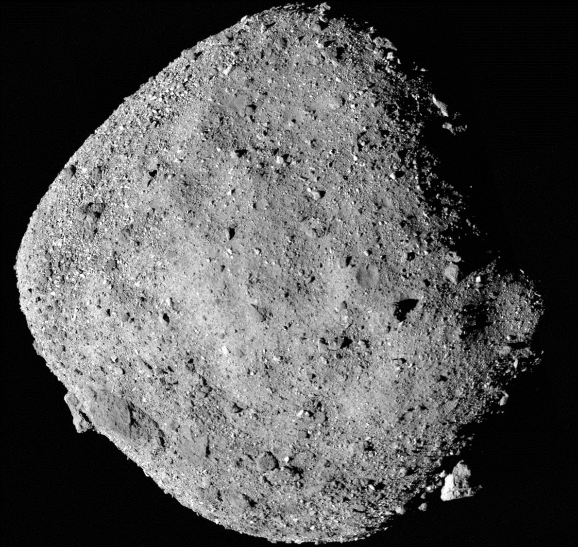
Figure 19.2 OSIRIS-Rex spacecraft
Image Credit: NASA

Figure 19.3 Return Capsule, imaged in flight on board the spacecraft
Image Credit: NASA
20: Red Rover - Lunokhod 1
Landing a rover or returning a sample from something small like a comet or asteroid is one thing; doing the same for a planet or a large moon is something else. The major problems are gravity, atmosphere and geology, all of which are specific to the place being visited.
So far, true rovers have only landed on the Moon and Mars.
The first rover vehicle was Lunokhod 1 (“Moon Walker 1”) - another first for the former Soviet Union. Launched on 10 November 1970, Luna 17 landed on the Moon on 17 November, and out rolled the rover a few hours after touchdown. The rover, a bit over one metre high and two metres across, was rather unkindly described in the Western press as the “Flying Bathtub”. With its eight wheels, and two forward and two reverse gears, it could get around at about 100 metres per hour, and was driven by remote control from a team of drivers back on Earth. The ‘lid’ of the rover was opened during the lunar day to expose the solar cells, and closed during the night to protect them.
The main function of the rover was to collect images (it sent back over 20,000 TV pictures and 206 high-resolution panoramas), and soil analysis using an x-ray fluorescence spectrometer. Being solar powered, it ground to a halt during the lunar night but, overall, it operated for 11 lunar days (about 11 months) before losing radio contact. Unfortunately, the ‘drivers’ were military specialists and measured success by the number of metres travelled, resolutely passing interesting-looking rocks and stuff that the scientists wanted to photograph.
On 8 January 1973, another Luna launch carried a slightly upgraded version, Lunokhod 2, which began rolling around from 16 January. In addition to studies of the lunar surface, it also made light and x-ray measurements to check out the viability of using the Moon as a site for an astronomical observatory. Moon Walker 2 only lasted four lunar days (four months). On the third day it drove into a crater, and the open lid scooped up some Moondust from the crater wall. At the end of the lunar day, the lid was closed, and the Moondust fell onto the thermal radiators lying directly underneath. After two weeks of hibernation, the lid was reopened, the rover came back to life, but died shortly afterwards when it overheated.
Figure 20.1 Lunokhod 1
Image Credit: NASA
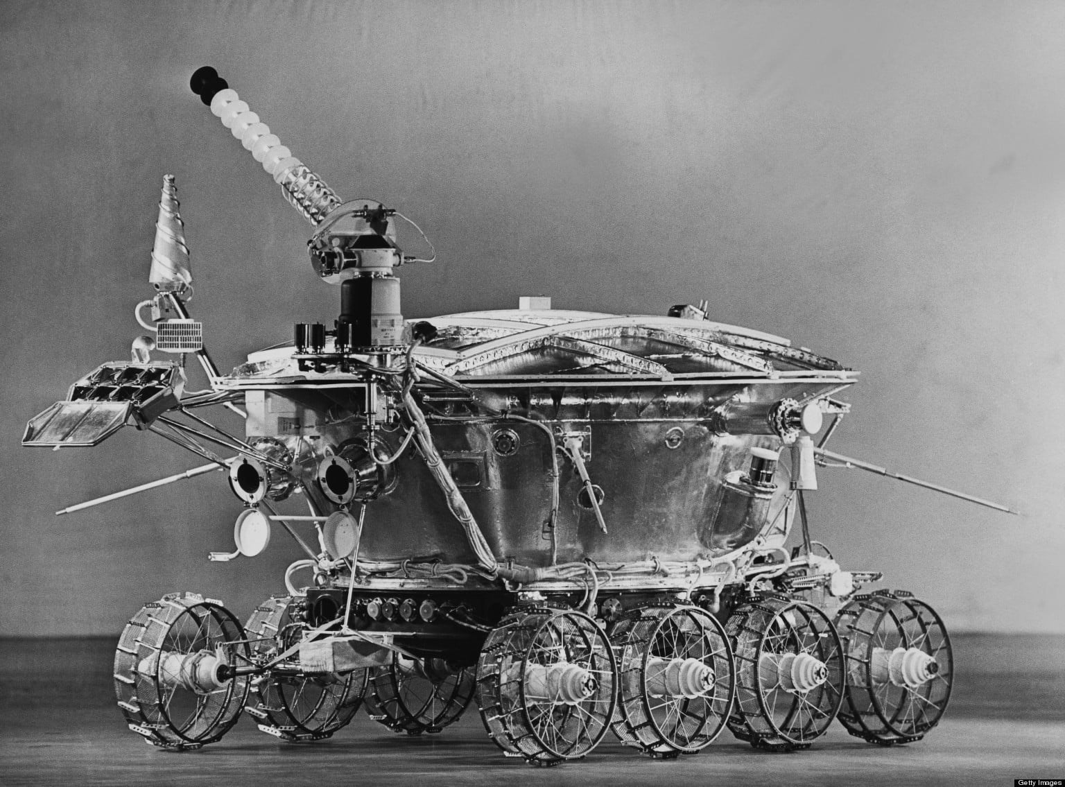
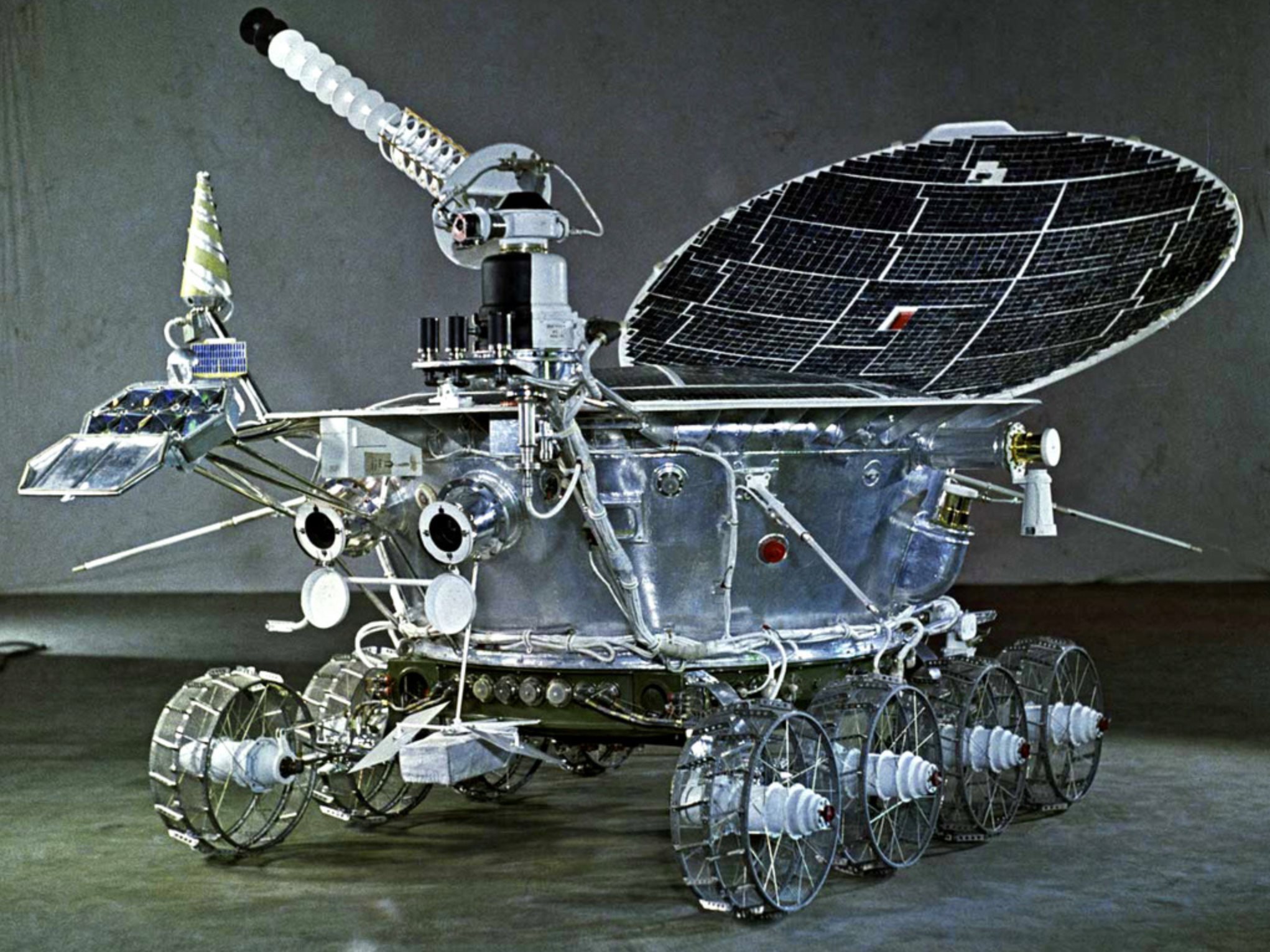
Figure 20.2 Model of Lunokhod 1 in roving mode, with the lid open to expose the solar cells
Image Credit: Demetreus Chryssikos
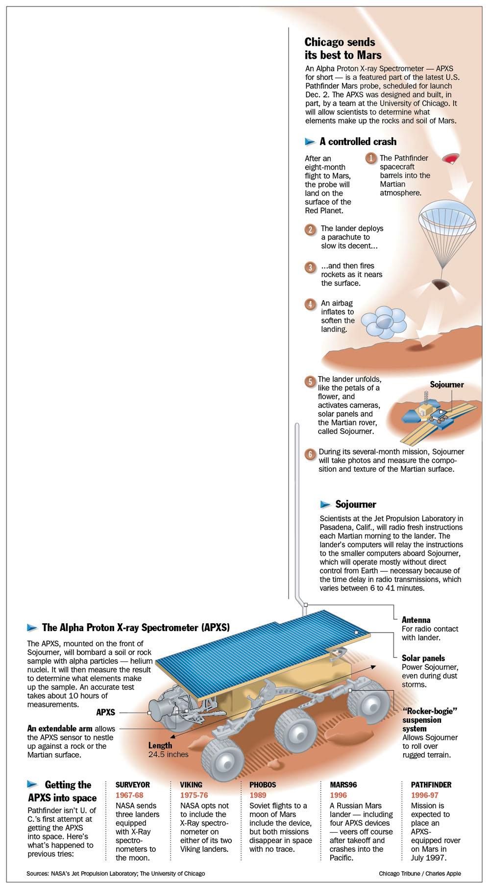
21: Red Planet Rover - Sojourner
I’m sharing another info-graphic from Charles Apple: covering Sojourner, it was produced before the launch. Sojourner is believed to be the first rover on Mars. Above, we met the USSR Prop-M rovers (the ski-mobiles) but we don’t know if one of them ever deployed because the parent lander craft stopped communicating.
Sojourner was actually launched on 4 December 1996. It began its sojourn on Mars on 5 July 1997, rolling away from its parent lander, Mars Pathfinder. It was semi-autonomous, receiving its daily marching orders from Earth but able to do some things autonomously (for example returning to home base if comms were lost). The machine sent back some useful chemical analyses of a number of rocks, and operated for nearly three months. During its time, it travelled a total of about 100 metres, keeping within 10 metres of Mars Pathfinder.
Figure 21.1 Sojourner
Image Credit: Charles Apple
22: Mars attack - Spirit and Opportunity
On 10 June 2003, a delta II rocket blasted off from Cape Canaveral carrying the latest NASA JPL mission to Mars. 27 days later, on 7 July, a second delta II rocket lifted off carrying the second of a pair of twins.
In January 2004, the celebrated pair of NASA rovers touched down on different sides of the planet, and Spirit and Opportunity began their road trips to give us unprecedented knowledge of the mineralogy and geology of Mars.
The 1.5m x 1.6m x 2.3m mobile machines carried cameras, thermal emission spectrometers (to rapidly identify rocks), Mössbauer spectrometers for details mineralogical analysis, x-ray spectrometers for chemical analysis of rocks, rock abrasion tools and magnets for picking up samples of the surface, and imaging microscopes to send back pictures of the grains of Mars dust they found. Anyone who was paying attention at the time will remember the gorgeous high-resolution images sent back from the surface of Mars, and the scientists would drool over the new data on mineralogy. The rovers even played amateur astronomer by imaging Mars’ tiny moons heading across the sky.
Target planning, route planning and ‘driving’ was done by a team at JPL. In total, 12 people have worked as rover drivers. They do not operate in real time due to the latency (it can take over 20 minutes for a command to travel from Earth to Mars), but set up a couple-of-days sequence of activities for the rover, which is uplinked via NASA’s Deep Space Network. The rovers had no autonomous capabilities, so good imaging was important so that the rovers’ routes could be planned to dodge rocks or other obstacles, as they travelled up to 100 metres per day (a Martian day is a bit longer than an Earth day).
Spirit lasted for 6 years and 9 months, rather longer than the original mission plan of 3 months. Opportunity boxed on, roving around and returning data, for 15 years. In the end, Spirit ‘froze’ to death after its power system fell short in providing power to keep it at a safe operating temperature, while Opportunity finally gave up when a planet-wide dust storm left its solar panels coated in dust.
Figure 22.1 Spirit rover
Image Credit: NASA
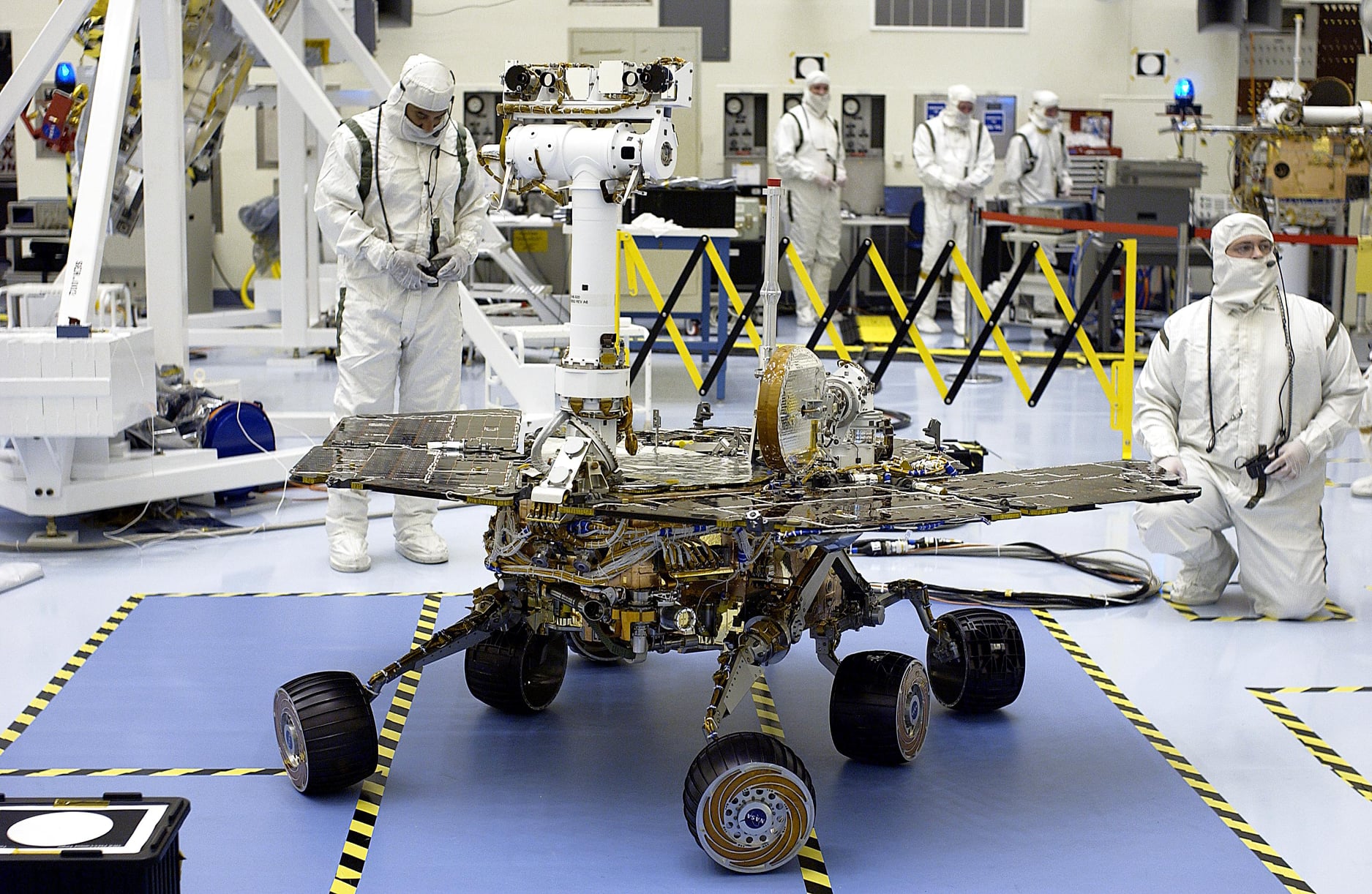
Figure 22.2 Panorama of “Fram Crater” from Opportunity
Image Credit: NASA
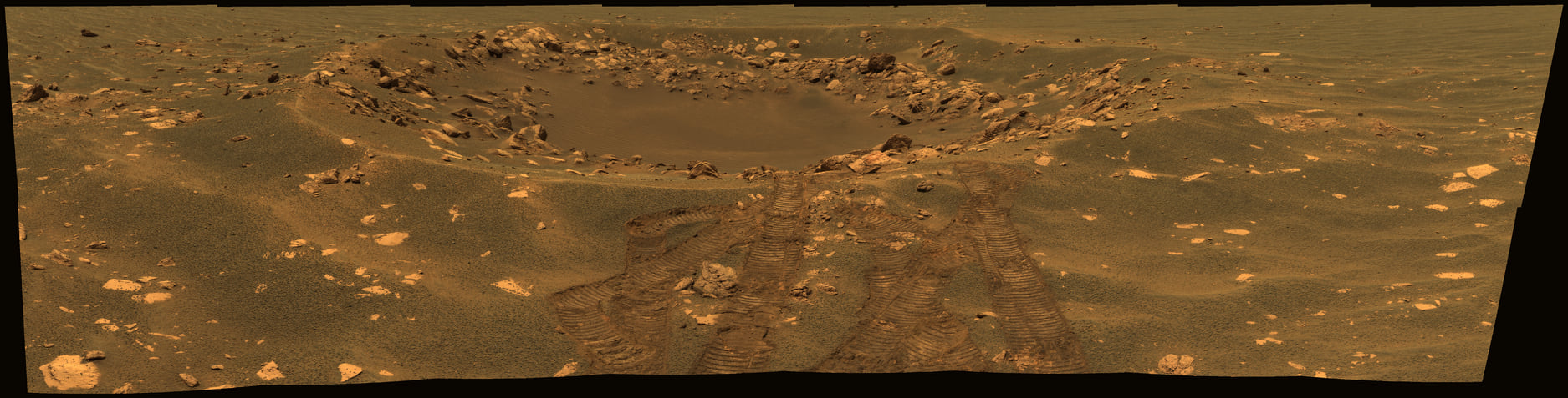
Figure 22.3 Some of the mission team at JPL: 2nd from left is Vandi Verma, one of the 12 rover drivers, who has driven three of NASA’s Mars rovers, at one of the mission-planning screens.
Image Credit: NASA

23: Rabbit in the Moon - Cháng’é
Since 2004, the China National Space Administration has been pursuing a program of Lunar exploration, intended to lead to a human landing on the Moon. On the way to this goal, the lunar lander 嫦娥三号 (Cháng’é 3) was launched from the Xichang Launch Centre in Zeuan Town (Sichuan) on 1 December 2013, using a 3-stage Long March 3B rocket. It landed using retro-rockets on 14 December 2013, and out rolled 玉兔 (Yùtù), the 140-kg, 1.5m-long rover vehicle. The rover carried twin cameras to take stereo images, x-ray and infrared spectrometers and, in a first for lunar exploration, a ground penetrating radar, able to image the subsurface down to 30 metres.
While Yùtù got busy exploring the lunar surface, the lander Cháng’é 3 deployed its ultraviolet telescope to carry out astronomical observations in the UV. The rover itself apparently had some difficulties coping with the temperature gradients caused by directly incident sunlight on one side, opposing the frigid darkness of space on the other. It did not live up to its mission plan of roving up to 10 km, though it continued communicating with Earth up until March 2015.
The next mission in the program was 嫦娥四 (Cháng’é 4), carrying another rover 玉兔二号 (Yùtù 2). Launched on 7 December 2018, this mission was rather more audacious, in targeting the far side of the Moon. It landed on 3 January 2019, and successfully communicated with Earth via a relay satellite sent into Lunar orbit for the purpose. The rover continues to rove and send back data, while the lander, among other things, tried hatching some seeds and insect eggs inside a small ‘biosphere’.
By the way Cháng’é is a mythological Moon goddess, and Yùtù (“Jade Rabbit”) is the Chinese name for the “Rabbit in the Moon".
Figure 23.1 Yùtù 2 rover on the Moon
Image Credit: China National Space Administration
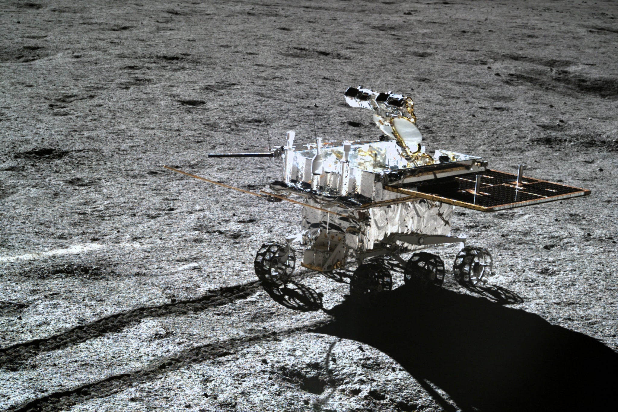
Figure 23.2 The first panorama from the far side of the Moon: The image shows Yùtù 2, shot from Cháng’é 4. See the image at full resolution here.
Image Credit: China National Space Administration

24: Rock and Roll - Curiosity
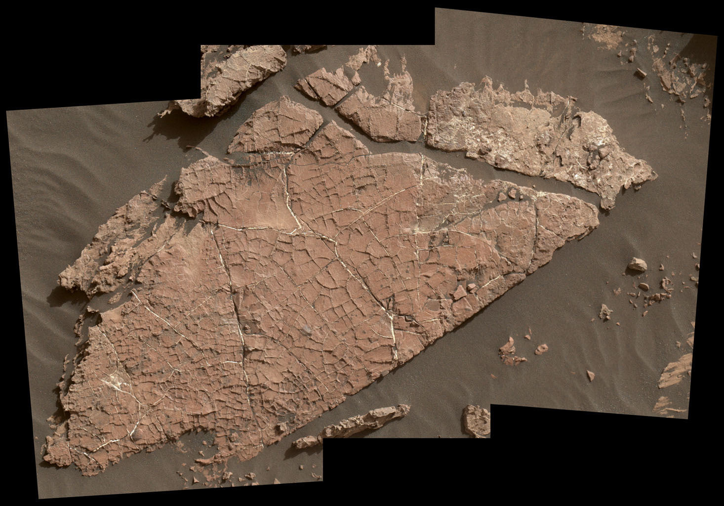
The last of the great rovers - the NASA/JPL rover, Curiosity - is seriously more significant than Spirit & Opportunity; larger, heavier, many more scientific instruments; cameras on a robotic arm that allow it to take ‘selfies’; Curiosity is pushing forward some serious science about the red planet. A recent (2020) science release showed evidence for dried-up lake beds on Mars - suggesting that in its past it was much more watery than it is today.
Figure 24.1 Infographic about Curiosity
Image Credit: Charles Apple

Figure 24.2 Photo of a possible dried lake bed on Mars
Image Credit: NASA
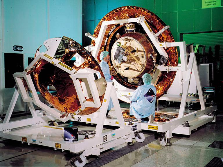
25: Ice sand, rivers of methane - Huygens
We’ve covered all the rovers, but I can’t move on without mentioning the total rock star of planetary landers - Huygens. Built for the European Space Agency, Huygens was part of the joint NASA-ESA Cassini Mission to Saturn, launched on 15 October 1997. On 14 January 2005 Cassini dropped the 320kg descender which planed (using a disposable heat shield) and then parachuted into the nitrogen-methane atmosphere of Titan, the largest moon of Saturn. The landing environment was unknown, and the probe was designed to send back about 30 minutes-worth of data after landing, either on solid ground or in an ocean.
It measured the density, thermal and electrical properties of the atmosphere (including listening for radio waves), as well as the wind speed. Its onboard gas chromatograph carried out chemical analysis at different altitudes, and the Surface-Science Package provided a number of measurements of the properties of the rocky surface where it landed. The detailed composition of the atmosphere even allowed some conclusions to be made about the internal geological structure of the moon. On top of all that, it sent back that stunning video of its descent, showing a world with mountains, streams and lakes.
Video: View a narrated video of the descent onto Titan here.
Figure 25.1 Huygens descender inside its heat shield
Image Credit: ESA
26: Weather report - Himawari
Ever wonder where those groovy ‘satellite pictures’ of the weather come from? Here in Australia ‘weather pictures’ originate with the Australian Bureau of Meteorology, and the most useful data comes from two geostationary satellites belonging to the Japan Meteorological Agency - Himawari 8 and Himawari 9. These two are positioned so they can image Japan, Australia, and all points in between - the JMA makes the data freely available for use by all. The multispectral cameras can image the entire continent with a resolution down to 0.5 km - and, as well as producing colour visual images, they can image into the infrared. They are particularly useful for monitoring cyclones, thunderstorms, ash and smoke, and fog & low cloud.
Himawari 8 was built by Mitsubishi Electric, and launched from the Tanegashima Space Centre on 7 October 2014, using a Japanese H-IIA rocket and has been sending data ever since.
Video: There is a very nice time-lapse sequence of Earth (featuring Australia) from the Himawari 8 geostationary satellite here.
Figure 26.1 Himawari 8 with solar panels and comms dish folded, for launch
Image Credit: Mitsubishi
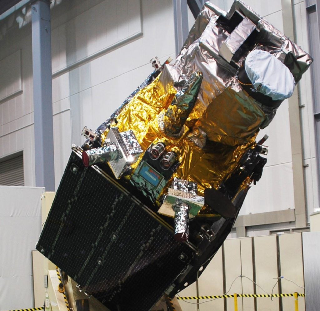
Figure 26.2 True colour image of Earth from Himawari 8
Image Credit: Wikimedia Commons

27: Moony McMoonface - Lunar Reconnaissance Orbiter (LRO)
The Lunar Reconnaissance Orbiter (LRO) carries a battery of scientific instruments to map the Moon in detail, from an eccentric polar orbit, dipping from about 160 km to just 20 km above the surface near the Moon’s south pole. At nearly two tonnes, it was launched on 18 June 2009, and was initially placed in a nearly circular orbit for its early mapping activities. Instruments on board include a cosmic-ray telescope (to measure life-threatening high energy radiation from space); a radiometer (to find areas which might be cold enough to trap water molecules); a Lyman-alpha mapper (to look for evidence of water molecules); a neutron detector (also to search for evidence of water ice); and three instruments to map the surface with unprecedented detail: a laser altimeter, a set of three cameras, and a radar ranger.
The machine and its instruments were designed and built in the US, and launched by NASA using an Atlas V rocket.
Among other things, the high-resolution mapping from LRO has allowed space archaeology: most of the landing sites and remaining debris from historic missions to the Moon have been found and photographed. It continues to operate and to return rather ambiguous data which is frustratingly not quite able to prove or disprove the presence of water in deep craters at the south pole. You can see some of the incredible high-resolution images of the Moon here.
Figure 27.1 Central peak of Tycho crater imaged by LRO
Image Credit: NASA
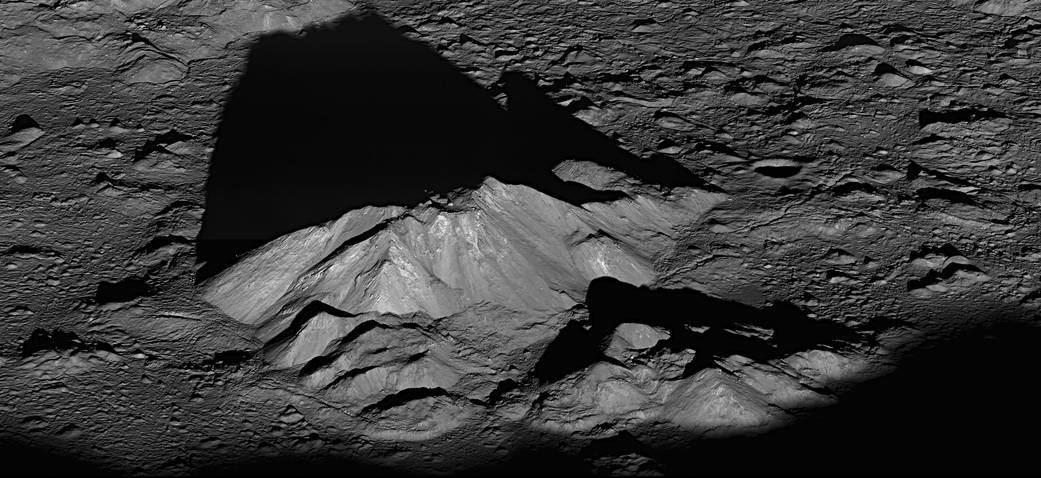
Figure 27.2 LRO with panels folded ready for launch
Image Credit: NASA

Figure 27.3 LRO image of the Apollo 11 Lunar module descent stage, on the Moon
Image Credit: NASA

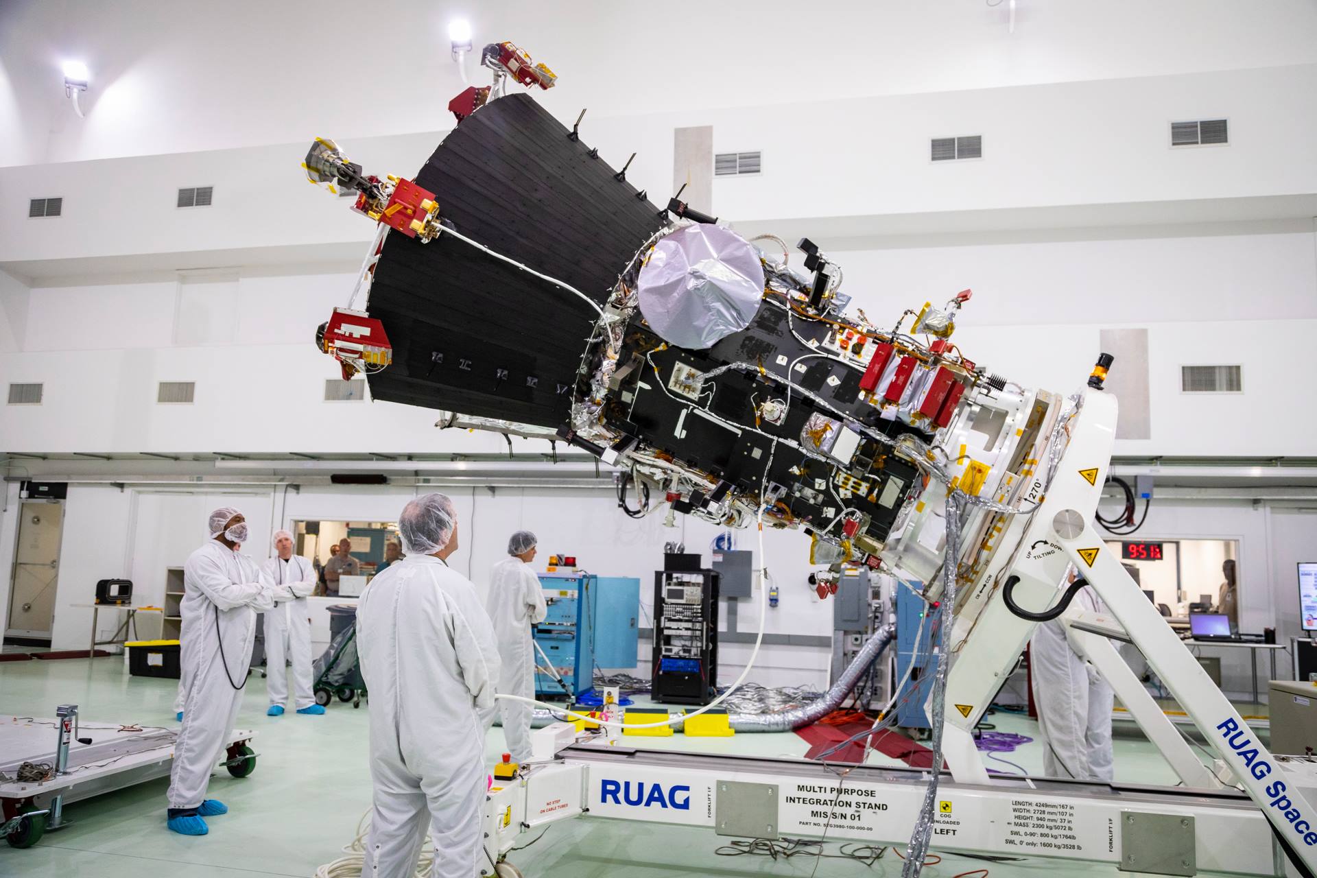
28: The Parker Solar Probe
The Parker Solar Probe (PSP) is the second-latest in a long line of spacecraft sent out to collect data on the Sun. This NASA mission, after being a political and budgetary football for decades, was launched on 12 August 2018 (a newer probe, the joint NASA/ESA Solar Orbiter was launched in February 2020). The PSP is designed to fly into the Sun’s atmosphere (the Corona) and measure the properties of the Corona and the electromagnetic fields in that region, which control the Solar Wind. Getting this close to the Sun is actually quite difficult for a number of reasons: firstly the heat, and secondly the orbital dynamics needed to drop so far into the ‘gravity well’, which requires the spacecraft to lose most of the kinetic energy it had when it left the Earth.
On the issue of heat, the PSP has a specially designed metal / ceramic heat shield to protect the scientific instruments on board. With orbital dynamics, its trajectory has been planned to repeatedly dip into the Solar atmosphere, then return high up into the vicinity of Venus, and use a planetary gravity assist to drop its periastron point progressively closer to the Sun. It will will dip closer and closer with each orbit, continuing for many years, thereby returning data from a range of heights and, each year, getting closer to in-situ measurements of the Sun’s atmosphere.
Video: View an animation of ‘interchange reconnection’ in the corona here.
Figure 28.1 PSP pre-launch
Image Credit: NASA
29: Can’t afford brakes - MESSENGER
As measured by ‘delta-v’ (basically energy consumption), Mercury is the most difficult planet in the Solar System to get to. It’s a bit like rolling down a massive steep hill on a bike, with the intention of stopping to inspect an interesting rock near the bottom. Only two spacecraft have been to Mercury, Mariner 10 in 1975 (though it stayed in solar orbit and didn’t try to get into Mercury orbit), and MESSENGER. There is another one on the way, ESA’s BeppiColombo, which was launched in 2018 and is due to arrive in 2025, after multiple gravity assists to provide ‘braking’.
NASA’s one-tonne MESSENGER spacecraft was launched on 3 August 2004, and arrived in March 2011, after using gravity assists from Earth, Venus and Mercury to shed kinetic energy. In addition to a suite of four cameras, it carried x-ray, neutron and gamma-ray spectrometers to analyse the mineralogy of the planet, a magnetometer to make detailed measurements of the magnetic field (discovered by Mariner 10), a laser altimeter to map the surface, a UV spectrometer to analyse the (very tenuous) atmosphere, and a plasma spectrometer to analyse radiation belts above the planet, induced by Mercury’s magnetic field.
The spacecraft orbited and sent back data for four years until, in 2015, it ultimately ran out of fuel for attitude correction and crashed onto the surface of Mercury. During its time, it provided magnetic field measurements which proved that Mercury has a liquid iron core, it showed evidence of old volcanoes on the surface and, most amazing of all, detected water ice in the bottoms of deep craters at the planet’s poles.
Figure 29.1 MESSENGER spacecraft with panels folded pre-launch
Image Credit: NASA

Figure 29.2 Surface of Mercury imaged by MESSENGER
Image Credit: NASA
30: New Horizons
Only one spacecraft has approached the dwarf planet, Pluto. NASA’s New Horizons was launched on 19 January 2006, and took nine years of travelling to reach its target, the ‘Pluto-Charon system’, on 14 July 2015. On the way, it got a gravity assist from Jupiter and, by luck, passed near the Main-Belt asteroid, 132524 APL, providing a chance for mission scientists to test the craft’s instruments, with photos of the 2.5-km asteroid being returned. Later came the observation of the major moons of Jupiter, and the planet itself during the gravity assist. But it was early 2015 when the machine was fully activated to earn its pay check - the observation of Pluto.
The spacecraft carried two optical cameras, a UV camera to analyse the atmosphere, a ‘dust counter’, an instrument to detect high-energy radiation, and a solar wind analyser. The most memorable achievement is the collection of high-res images of the surface of Pluto, revealed to be mostly frozen nitrogen, with traces of methane and carbon monoxide. After completing this mission, the craft continued out into the Kuiper belt, and collected data on an object called ‘Ultima Thule’ lately renamed 486958 Arrokoth. New Horizons showed that it is made mostly of water ice with a variety of odd organic and nitrogen-bearing chemicals.
Figure 30.1 New Horizons spacecraft
Image Credit: NASA

Figure 30.2 New Horizons’ image of Pluto and Charon
Image Credit: NASA
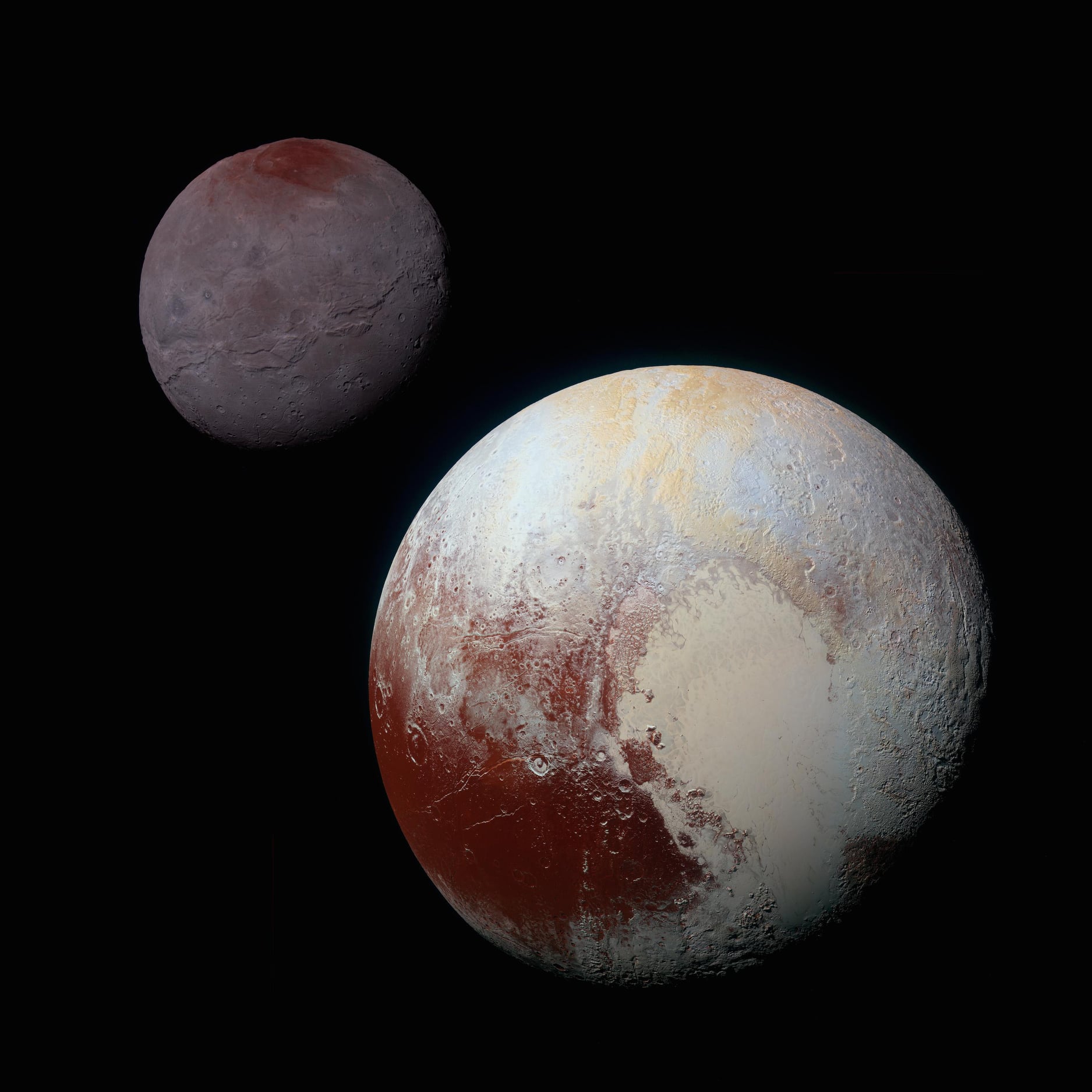
Figure 30.3 486958 Arrokoth, imaged by New Horizons
Image Credit: NASA

31: We are sailing - IKAROS and Akatsuki
One way to save on carrying rocket fuel is to use planetary gravity assists. Another is to harness the radiation from the Sun. This is often done by using solar panels to power an ion drive, but there is another way: harness the photon pressure directly using a sail!
IKAROS became the first sailing ship to reach another planet, when it zoomed past Venus in 2010, returning data on interplanetary dust, and gamma radiation. The sail incorporated LCDs, and operators were able to adjust the sail without using the rigging, but just by turning the LCDs on and off, thereby changing the reflectivity of the sail. The craft was a fairly hefty 300 kg, of which two kilograms was the sail, which measured 14 metres square when unfurled. After the sail was deployed, IKAROS took a selfie picture using a throwaway camera.
IKAROS was built and launched by the Japanese Space Administration, and was one of two Venus probes launched with the same H-IIA rocket. The second craft, Akatsuki, was a more conventional spacecraft equipped with five cameras, operating at wavelengths from UV to infrared, to study the atmosphere of Venus. An engine fault meant that when the craft arrived at Venus, it failed to get enough impetus to go into orbit, and the mission staff had to wait for five years for it to coast around the Sun and catch up with Venus again so they could try again. The craft has orbited Venus and sent back important information on the dynamics of the atmosphere ever since.
Figure 31.1 IKAROS's selfie: The spacecraft is the cylinder rigged in the middle of the square sail.
Image Credit: JAXA
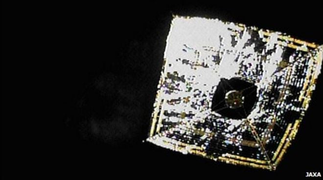
Figure 31.2 Akatsuki with solar panels folded for launch
Image Credit: JAXA

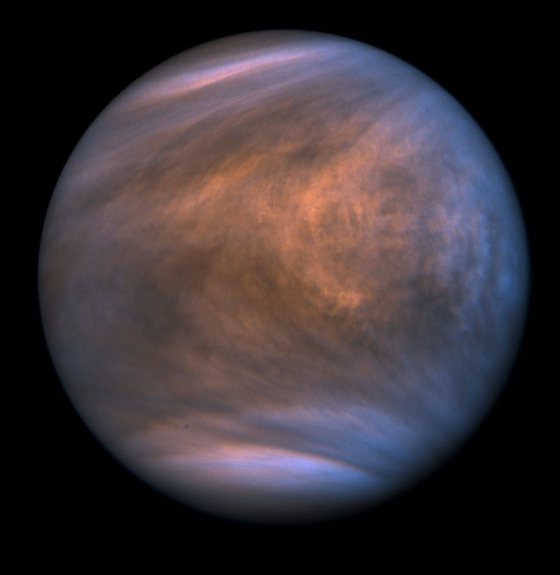
Figure 31.3 Image of Venus from Akatsuki UV camera
Image Credit: JAXA
32: Galileo (Figaro?)
Quite a few spacecraft from Earth have visited Jupiter - en route somewhere else to to get Gravity assists, but only two have orbited the giant planet.
The big one, which made a lot of discoveries about Jupiter and especially its moons, was Galileo, a US-led international effort launched by NASA in the cargo bay of the Shuttle Atlantis, on 18 October 1989.
It was a biggie - over two tonnes’ mass and over six metres tall. After the Challenger disaster, liquid fuel rockets were banned from the Shuttle cargo bay, so Galileo had to go up with a solid fuel booster and use multiple gravity assists from Venus and Earth to get to Jupiter in December 1995. It visited a couple of main belt asteroids on the way, and one of its photos revealed ‘Dactyl’ the tiny moon of asteroid 243 Ida.
Galileo orbited Jupiter in a set of eccentric orbits, which enabled it to approach some of the moons, and to limit its time in the destructive radiation belts near the planet. Among other things, Galileo provided evidence of the magnetic field of Ganymede, the volcanoes on Io, the subsurface ocean on Europa, and the giant plasma tail linking Io to Jupiter’s atmosphere. It made measurements of the magnetosphere of Jupiter, observed ammonia clouds in the atmosphere, and collected more data by dropping a 300kg descent probe into Jupiter. Even before arriving it had collected data on the planet by observing the impact of Comet Shoemaker-Levy 9.
Figure 32.1 Galileo with its descender
Image Credit: NASA
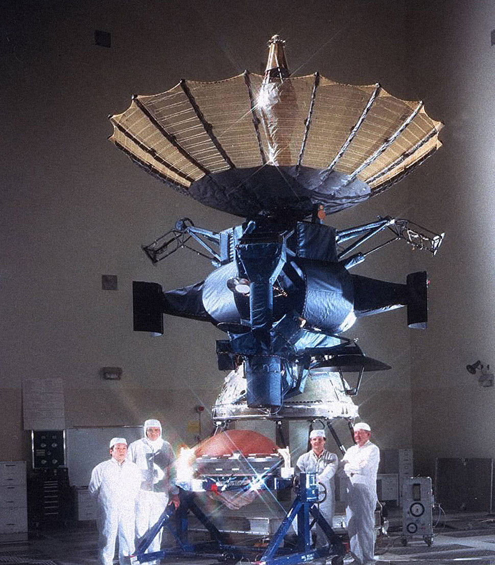
Figure 32.2 Evidence of movement of ‘ice rafts’ on Europa
Image Credit: NASA
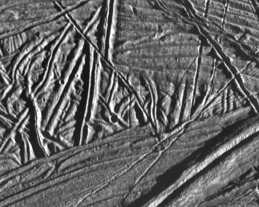
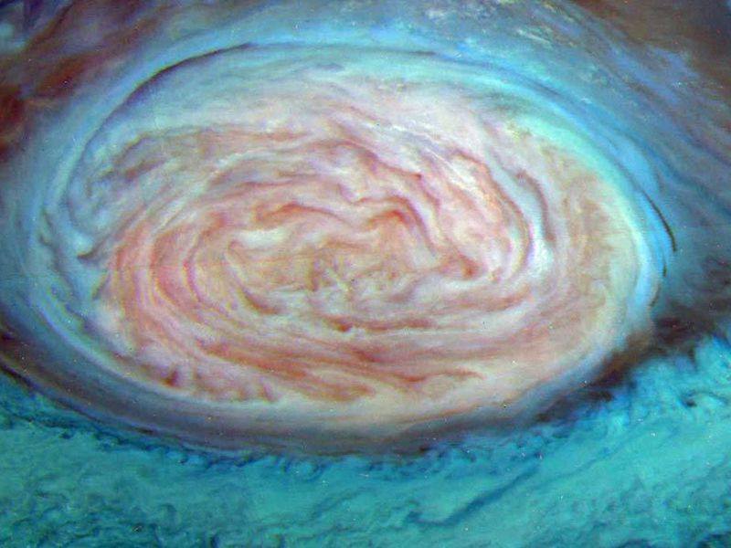
Figure 32.3 Great Red Spot of Jupiter, imaged by Galileo’s IR camera
Image Credit: NASA
33: Mars - Mangalyaan (MOM)
There have been a couple of great remote sensing missions to Mars, most notably NASA’s Mars Reconnaissance Orbiter (MRO) which they initially thought had found evidence for flowing water (2015) but later realised hadn’t (2017), and ESA’s Mars Express, which produced pretty strong evidence for a subsurface lake (2018). But here is a lesser known mission: the Mars Orbiter Mission (MOM) from the 4th space agency to reach Mars; after NASA, the Soviet Union, and ESA, came ISRO, the Indian Space Research Organisation.
Mangalyaan - known in English as “MOM” - was launched on 5 November 2013, on top of an Indian designed-and-built PSLV C25 rocket (normally used for launching polar satellites), from the Satish Dhawan Space Centre in Andhra Pradesh. It reached Mars on 24 September 2014 and was given a highly elliptical orbit varying from 420 km to 77,000 km high.
The 1.3 tonne spacecraft carried a Lyman-alpha photometer to study hydrogen in the Mars atmosphere, a methane sensor, a particle mass analyser to study the near-space environment of Mars, and infrared and optical cameras to map the surface and Mars’ two moons. A successful mission with a lot of scientific data returned and contributed to the international scientific literature. The original mission plan was for six months of operation, but the craft is still orbiting and sending back data today, nearly six years later.
Figure 33.1 MOM spacecraft being mounted on the launch vehicle
Image Credit: ISRO

Figure 33.2 Mars imaged by Mangalyaan
Image Credit: ISRO
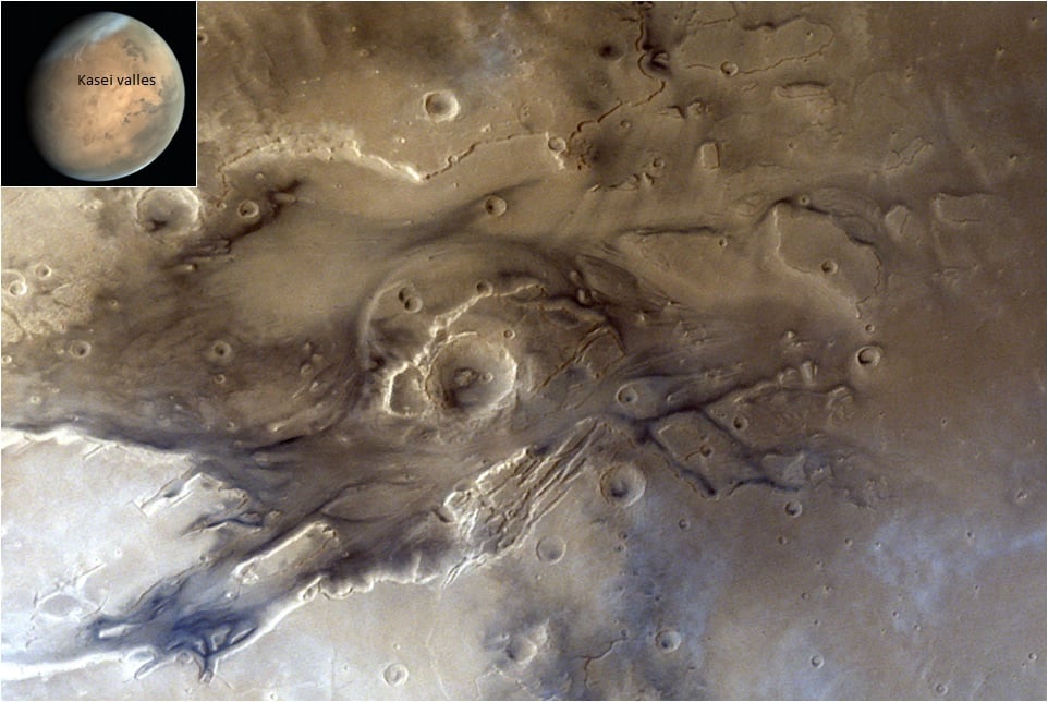
Figure 33.3 Mars imaged by Mangalyaan
Image Credit: ISRO
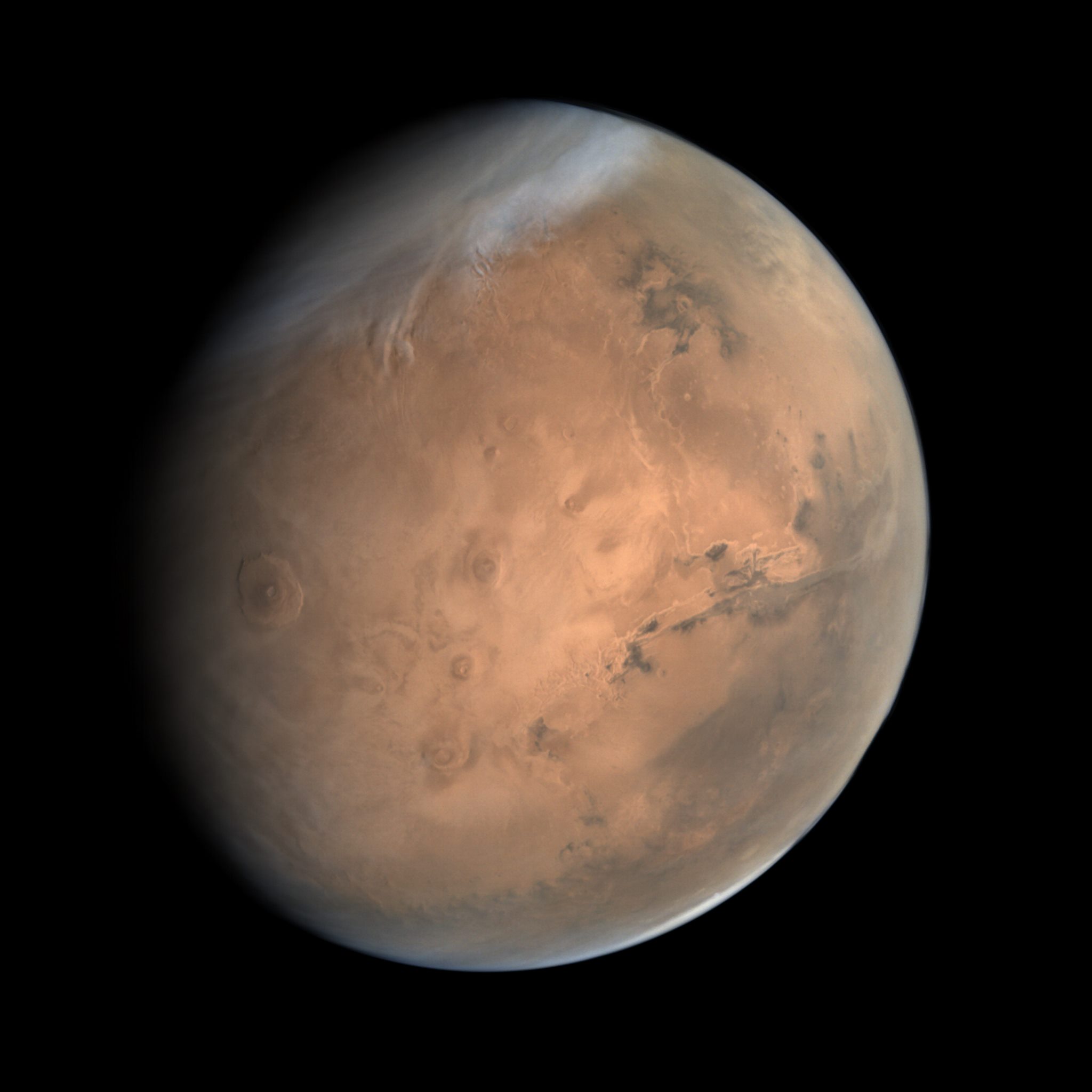
Figure 33.4 Commemorative banknote
Image Credit: A. Chandrakant

33: Ring me - Cassini
Only one spacecraft from Earth has orbited Saturn: Cassini, a collaboration of NASA, ESA and ASI (the Italian Space Agency). Launched on 15 October 1997, it used gravity assists from Venus, Earth and Jupiter to get to Saturn on 1 July 2004. It then spent 13 years collecting data and images of Saturn, its ring system, and its many moons. It made many discoveries about Saturn's moons and, of course, it was Cassini that carried the Huygens lander which descended to the surface of Titan.
Cassini was loaded with scientific equipment: visible, infrared and ultraviolet spectrometers and imagers to analyse the surfaces of the moons and compositions of atmospheres, a plasma spectrometer, mass spectrometer and dust analyser to analyse interplanetary materials in the region of Saturn, three instruments to measure electromagnetism near the planet, and radar for mapping solid surfaces. All this hardware plus the support infrastructure including the ability to transmit back to Earth was powered (possibly slightly controversially) by three plutonium-fuelled RTGs, as it was found not feasible to use solar panels at its working distance from the Sun.
Cassini imaged the rings of Saturn in unprecedented detail, and gave us a lot of new information on the 3-dimensional structure of the rings, including shepherd moons, propellor moons, spokes, and 3D spiral density waves. It sent back images of a massive storm on the planet following the breakup of the ‘great white spot’, and travelled around the poles to send back information on the evolution of Saturn’s ‘polar hexagon’.
At the end of its mission, as it ran low on fuel, the decision was made to dump the two-tonne, 7m x 4m probe into Saturn, to ensure that its wreckage would not contaminate any of the moons, many of which are under active consideration for hosting water-based life. It sank into the great planet on 15 September 2017.
Figure 34.1 Cassini probe assembled
Image Credit: NASA
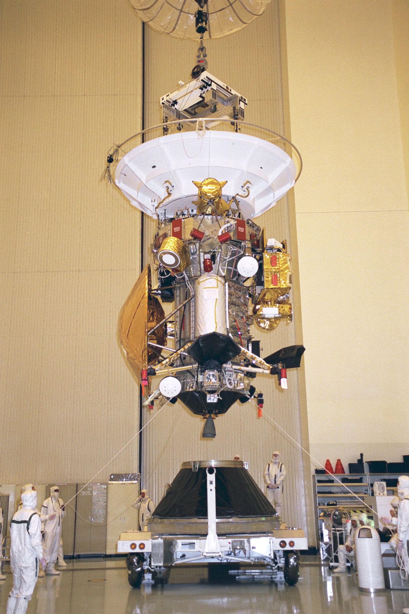
Figure 34.2 Northern hemisphere of Saturn, including the hexagon
Image Credit: NASA
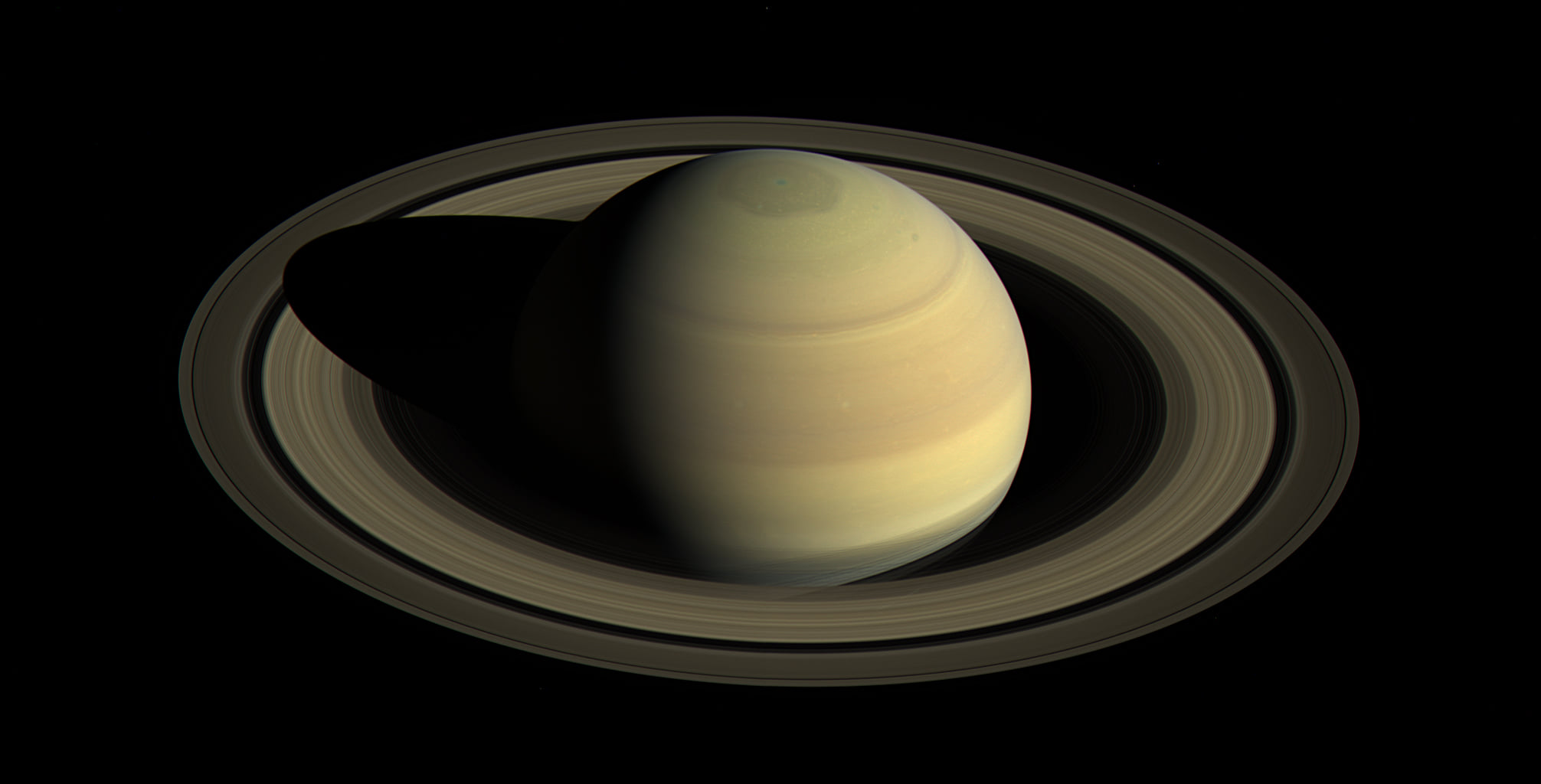
Figure 34.3 Giant storm
Image Credit: NASA
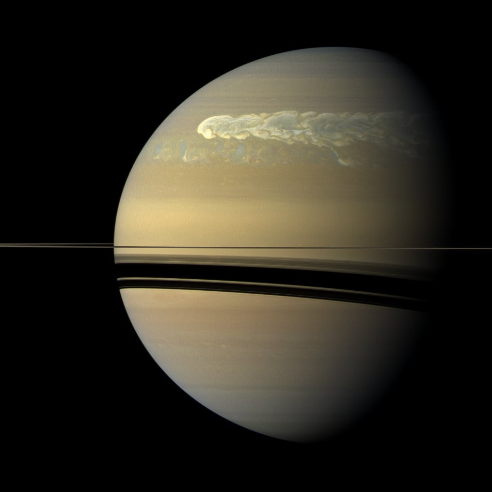
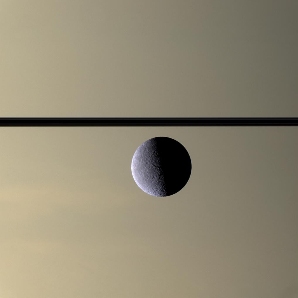
Figure 34.4 Rhea: The Cassini spacecraft looks toward Rhea’s cratered, icy landscape with the dark line of Saturn’s ringplane and the planet’s murky atmosphere as a background.
Image and Caption Credit: NASA
35: Interstellar - Voyager 2
In the early ’60s, it was realised that a chance alignment of the outer planets in the late ’70s would allow a single spacecraft to visit Jupiter, Saturn, Uranus and Neptune. Various options were considered, using combinations of different spacecraft (at different costs, etc.) but, in the end, the Voyager 2 mission was set up to do it.
As early exercises in technology qualification, Pioneer 10 (launched 2 March 1972) was sent to Jupiter, and Pioneer 11 (launched 6 April 1973) was sent to Jupiter and Saturn. Having gained this, experience Voyager 1 and Voyager 2 were set up for the grand tour mission. Voyager 2 was launched first, on 20 August 1977. Voyager 1, launched on 5 September 1977, was a backup mission, able to take over in case Voyager 2 ‘failed to reach orbit’. But knowing that Voyager 2 was off and running, Voyager 1 was dedicated to the second string mission, which was optimised to visit Saturn’s largest moon, Titan.
Voyager 2 encountered Jupiter on 9 July 1979, Saturn on 26 August 1981, Uranus on 24 January 1986, and Neptune on 25 August 1989. At the time, the data from Jupiter and Saturn were a revelation, but the results have been superseded by Galileo and Cassini. But Voyager 2 remains the best source of in situ data on Uranus and Neptune. As usual, the 800-kg craft was loaded with multispectral cameras, IR and UV spectrometers, magnetometers, ion gauges and cosmic-ray detectors. It produced the stunning photos of the moons of Uranus and Neptune, which we met in Part 8b, as well as providing the first really close-up data on the two outer gas giants.
Voyager 2 left the Solar System and entered interstellar space on 5 Nov 2018. Its twin, Voyager 1, taking a different trajectory, passed the heliopause and entered interstellar space six years earlier on 25 August 2012, and is currently the most distant Earth-built object. Pioneer 10 and Pioneer 11 also have enough speed to reach interstellar space and, one day, so will New Horizons. Voyager 2 is headed in the general direction of Sirius, which it might reach in about 300,000 years.
The Voyager craft carried metal analogue recordings of music (us old people call them “LPs”) from a variety of human cultures. Here is a list of the music on the voyager records. It’s worth an hour or two on youtube to track them down!
Figure 35.1 Voyager 2 spacecraft
Image Credit: NASA
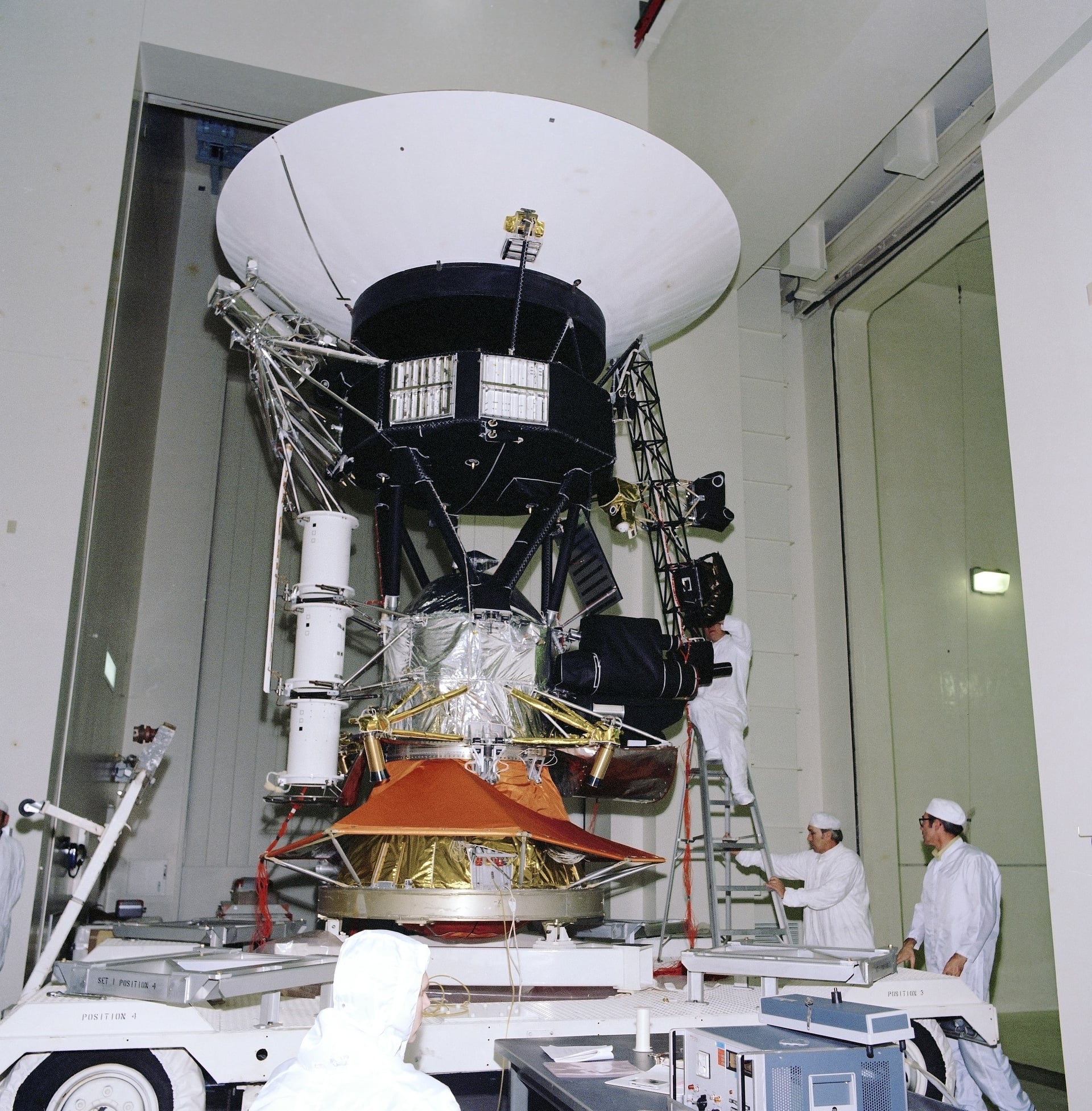
Figure 35.2 Uranus imaged by Voyager 2
Image Credit: NASA
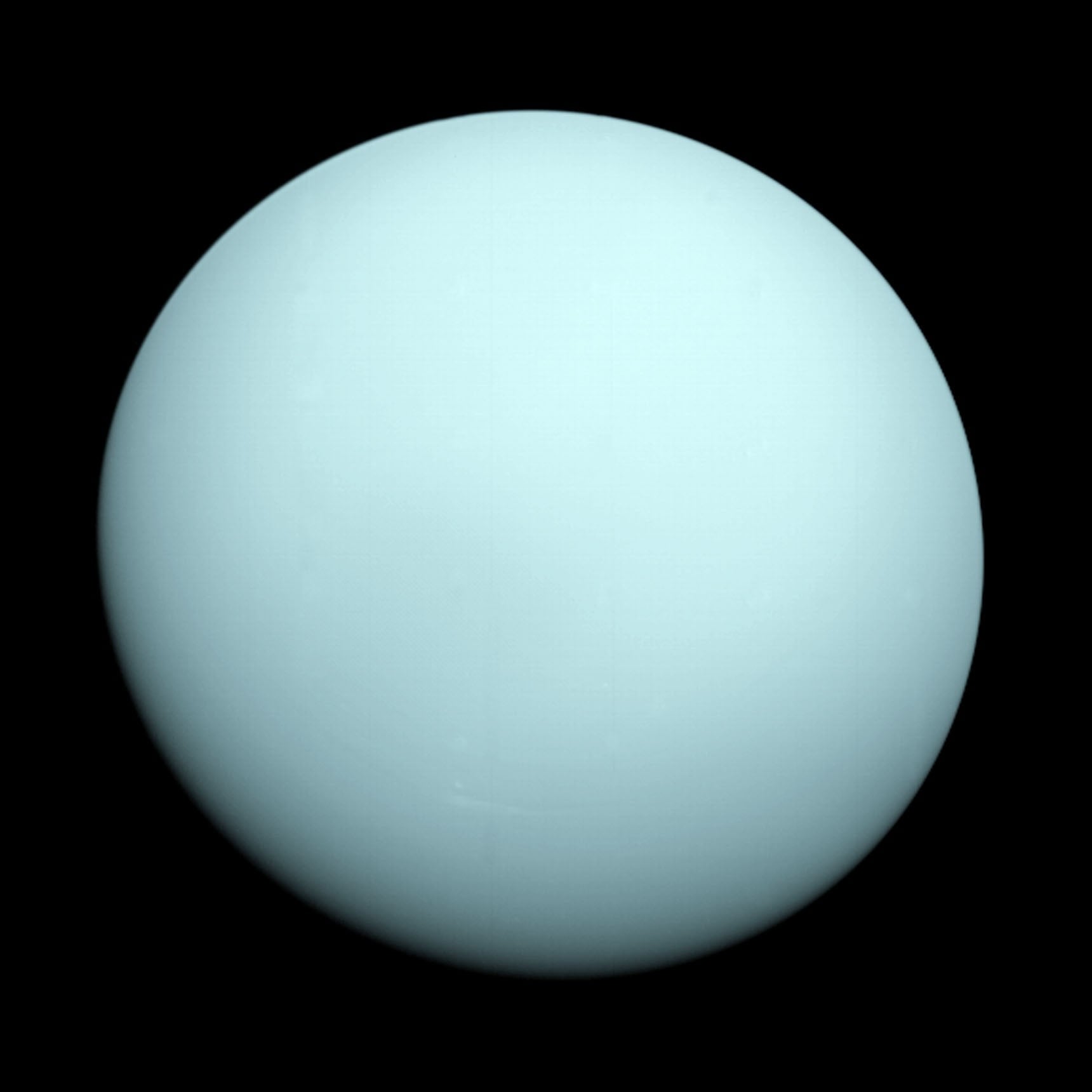
Figure 35.3 Neptune imaged by Voyager 2
Image Credit: NASA

Figure 35.4 Plot of trajectories of Voyagers 1 and 2
Image Credit: NASA

36: Juno
On 5 August 2011, NASA Launched an Atlas V551 rocket carrying Juno, a spacecraft specifically designed to explore Jupiter. Using a gravity assist from Earth, the machine reached Jupiter orbit on 5 July 2016. Juno was well armed with an array of scientific instruments selected to collect detailed information on the largest planet in our Solar System. It was not about discoveries, more about detailed in-situ measurements to really understand the radiation belts, the electromagnetic environment, and the distribution of mass inside Jupiter.
Juno is still orbiting Jupiter and sending back data. It has enough fuel for attitude control to see it into 2021, and the plan is to dump it into Jupiter when the fuel runs out. With spacecraft, one of the key decisions is how to power it. It depends on the distance and the requirements of the science payload and the comms, etc.: and NASA’s solar panels are the world’s best high-efficiency ones, not like the ones on your roof! In fact, Juno is the first Jupiter mission to use panels - all previous outer-solar-system craft have used RTGs. By the way, Saturn’s orbit has nearly double the radius of Jupiter’s - so there is a factor of four in the insolation going out to the cold outer reaches that Saturn inhabits.
RTG = Radio-isotope thermal generator. This type of nuclear power plant has (usually) a plutonium core to generate heat. It is surrounded by a bunch of thermocouples (made of relatively cheap wire) that use the temperature to generate electricity. Most of the power of the RTG comes out as heat which has to be dumped from the spacecraft - usually a special radiator panel is attached to do this.
Figure 36.1 Juno spacecraft
Image Credit: NASA
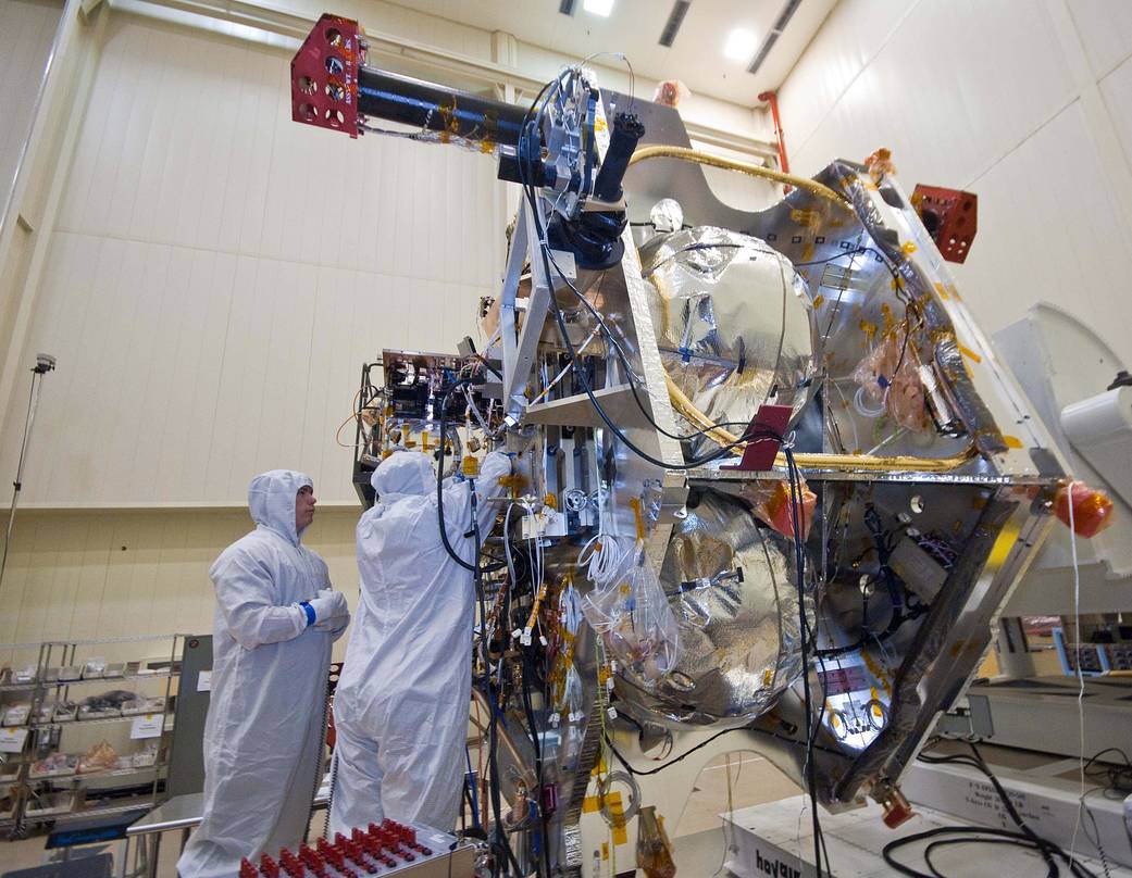
Figure 36.2 Infographic
Image Credit: Charles Apple
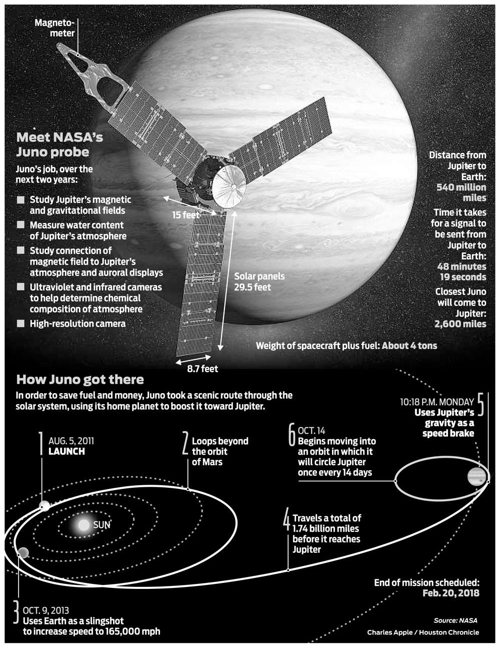
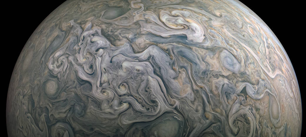
Figure 36.3 Juno image of the atmosphere of Jupiter
Image Credit: NASA
37: Intergalactic - GALEX
For astronomers, it is quite difficult to make observations in ultraviolet light (UV) because most of it is absorbed by the upper atmosphere. But UV light is good for observing galaxies - bright UV emission is an indication of star formation and UV measurements are very useful in understanding the life history of galaxies.
This is the scientific rationale for the “Galaxy Evolution Explorer” - GALEX - a space-based UV telescope. Its mass is 280 kg, it is about two metres tall by one metre across (three metres across with the solar panels), and was sent into Earth orbit on 28 April 2003, with enough fuel to do attitude corrections for about 12 years. It was decommissioned in June 2013 after carrying out sky surveys and building up a database of UV brightnesses and spectra of galaxies over most of the sky. Although no longer sending data, it will continue in orbit for about another 50 years before being caught by the atmosphere and burning up.
If you want to do some astronomy using GALEX, you can access all of its data here.
Figure 37.1 GALEX UV space telescope
Image Credit: NASA

Figure 37.2 The star MIRA is travelling so fast it creates a shockwave in interstellar gas.
Image Credit: NASA
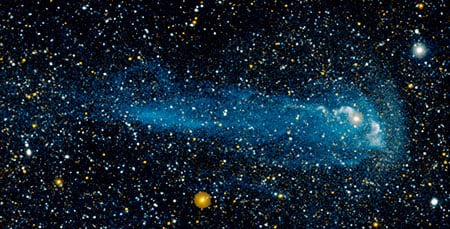
Figure 37.3 NGC 253: The Silver Dollar Galaxy, NGC 253, imaged in UV by GALEX - the wisps of blue represent relatively dustless areas of the galaxy that are actively forming stars. Areas of the galaxy with a soft golden glow indicate regions where the far-ultraviolet is heavily obscured by dust particles.
Image Credit: NASA/JPL-Caltech
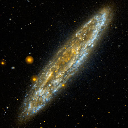
Figure 37.4 Shells of gas ejected from a star (Z Cam) when it exploded as a supernova
Image Credit: NASA

38: More planets than stars - Kepler
On 7 March 2009, a Delta II rocket blasted off from Cape Canaveral carrying a one-tonne telescope with a 1.4m-diameter mirror, which was delivered into solar orbit, approximately trailing the Earth in its orbit. It had an unusual mission: to stare at a small patch of sky away from Earth and away from the Sun, and measure the brightness of about 150,000 stars, continuously for years, using repeated 6.5-hour exposure times.
The purpose of the Kepler telescope is to find planets orbiting other stars - well, not by imaging them directly, but by measuring the tiny dip in brightness of a star when a planet passes in front of it. It collected this photometric data for four years, until failures in its ‘reaction wheels’ meant that it could no longer point on target (the scope needs to turn as it rotates in orbit, to keep staring at the same point in the sky). The mission scientists then continued to collect data, using Kepler to spot supernovae, asteroids and comets, until it ran out of fuel in 2018.
During its four-year primary mission, Kepler made repeat observations of stars and identified over 1200 planets. Based on this sample, it’s estimated that a galaxy like the Milky Way has more planets than stars. You can look through the Kepler database here (it’s now being extended by a new spacecraft called TESS).
Figure 38.1 Kepler space telescope
Image Credit: NASA
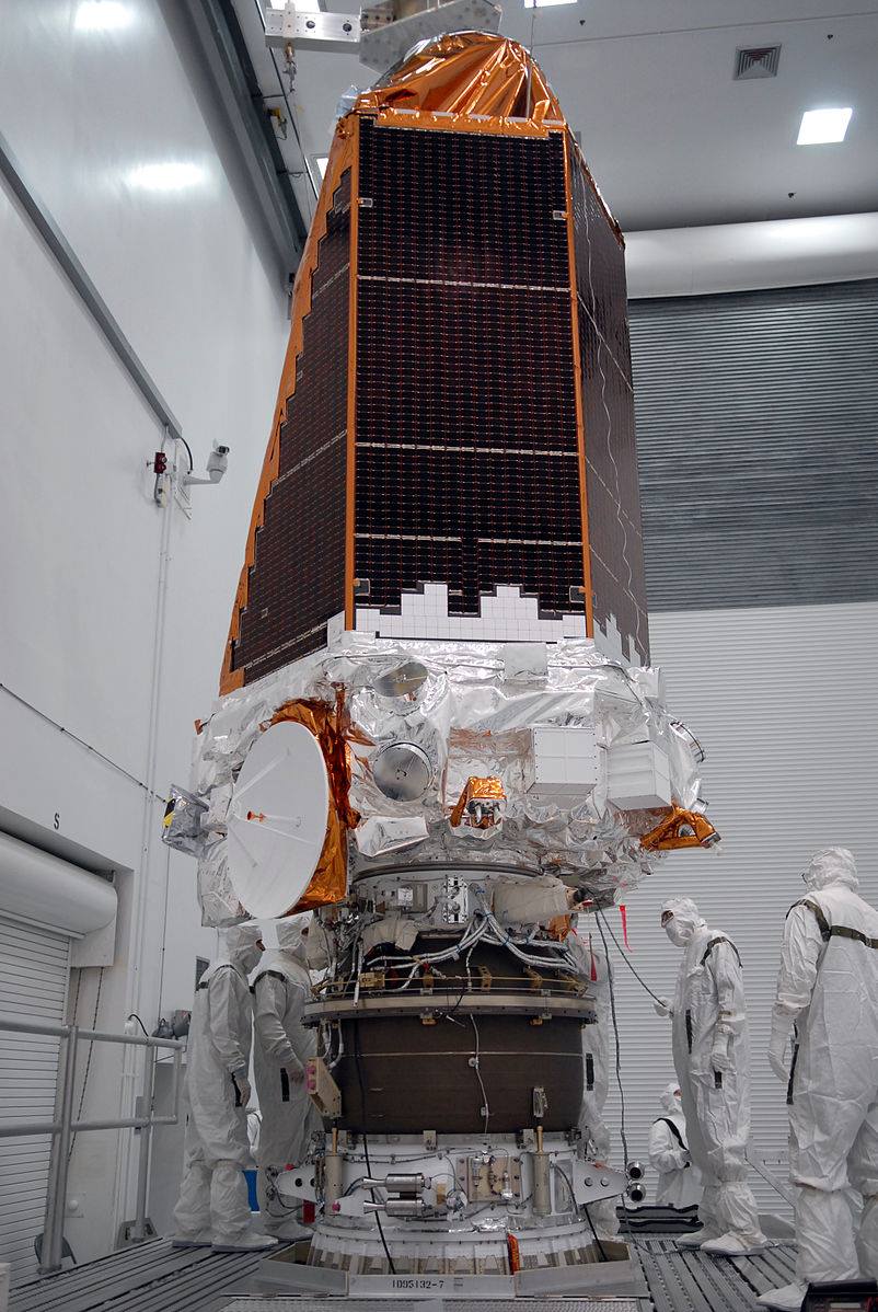
Figure 38.2 Size distribution of planets found by Kepler
Image Credit: NASA
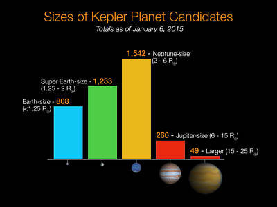
Figure 38.3 Kepler star field
Image Credit: NASA

39: 3K - WMAP
Starting in 2003, a series of papers published by a joint team from Johns Hopkins University, Princeton University and NASA have become some of the most highly-quoted papers in physical science. Members of the team were awarded the Shaw prize in 2010, the Gruber prize in 2012, and the Breakthrough prize in fundamental physics in 2018. The results came from a nine-year mission (2001-2010), in which the entire sky was mapped by a spacecraft carrying microwave receivers, travelling in solar orbit near the Earth’s ‘trailing’ L5 Lagrange point. Initially called “MAP”, the craft was renamed “WMAP”, the Wilkinson Microwave Anisotropy Probe, in 2003.
WMAP’s achievement has been to provide a highly accurate map of fluctuations in the cosmic microwave background radiation. These are very small variations in temperature which retain an imprint of the hot particles which existed when the first atoms formed as the universe cooled following the ‘Big Bang’. As the universe has continued to expand and cool, that early fireball is now just 3 degrees above absolute zero.
One of the early puzzles in cosmology is why the background is so smooth - and the theory of ‘cosmic inflation’ was put together to explain it. Not many people like it, but it seems to be the only logical way of explaining what we observe. Results from WMAP have played the major role in quantitatively establishing what the universe is made of: its data can really only be explained if the universe is 13.8 billion years old, expanding at a rate of 69.3 km/s/Mpc, and is made of 4.63% matter, 24.02% dark matter, and 71.35% dark energy.
If you want to check the calculations for yourself, all of WMAPs data is online, start here.
Figure 39.1 Temperature map of the sky, after 9 years of observation
Image Credit: NASA

Figure 39.2 WMAP spacecraft
Image Credit: NASA
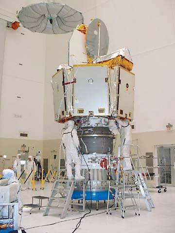
Figure 39.3 Model of WMAP as deployed
Image Credit: NASA

39: IR - Spitzer
Above, we saw Kepler, the famous exoplanet hunter. But, remember that Kepler only looked at a tiny patch of the sky and, as it used the transit method, it could only spot planets crossing the disk of the stars during its four years of operation. If studying our own Solar System, it would be unlikely to spot Saturn (29 year orbit) or even Jupiter, with its 12-year orbit.
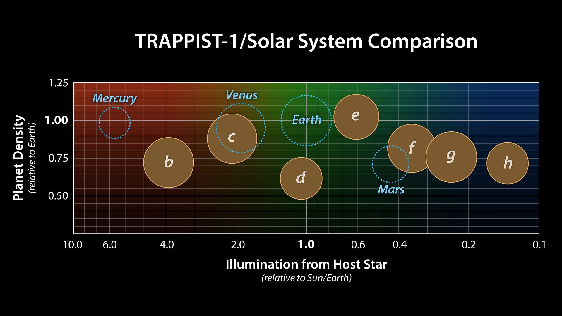
But there are other space telescopes that have found exoplanets. In 2005, the Spitzer space telescope (2003-2020) actually measured infrared radiation coming from two exoplanets - the first time planets had been directly detected. In 2016, it discovered five of the seven planets known to orbit the star Trappist-1, a red-dwarf star nearly 40 light years away: all its known planets are rocky and roughly Earth-sized.
When the Spitzer space telescope was launched, and put in Earth-trailing solar orbit, there was no idea of using it as a planet hunter. Its three infrared instruments were intended to study galaxy formation, cold stars and planet formation from dusty disks. The telescope was used for a while hunting exoplanets after its liquid helium coolant ran out (the IR instruments need to be kept cooler than the things they are observing), but shut down earlier this year. Astronomers are keenly awaiting the next great IR telescope, the James Webb, which is under construction.
Figure 40.1 Star formation in the “Stellar Snowflake Cluster”
Image Credit: NASA
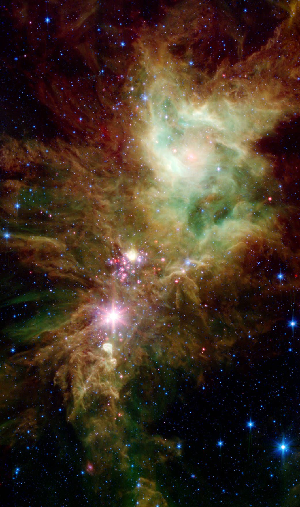
Figure 40.2 Spitzer Space Telescope
Image Credit: NASA
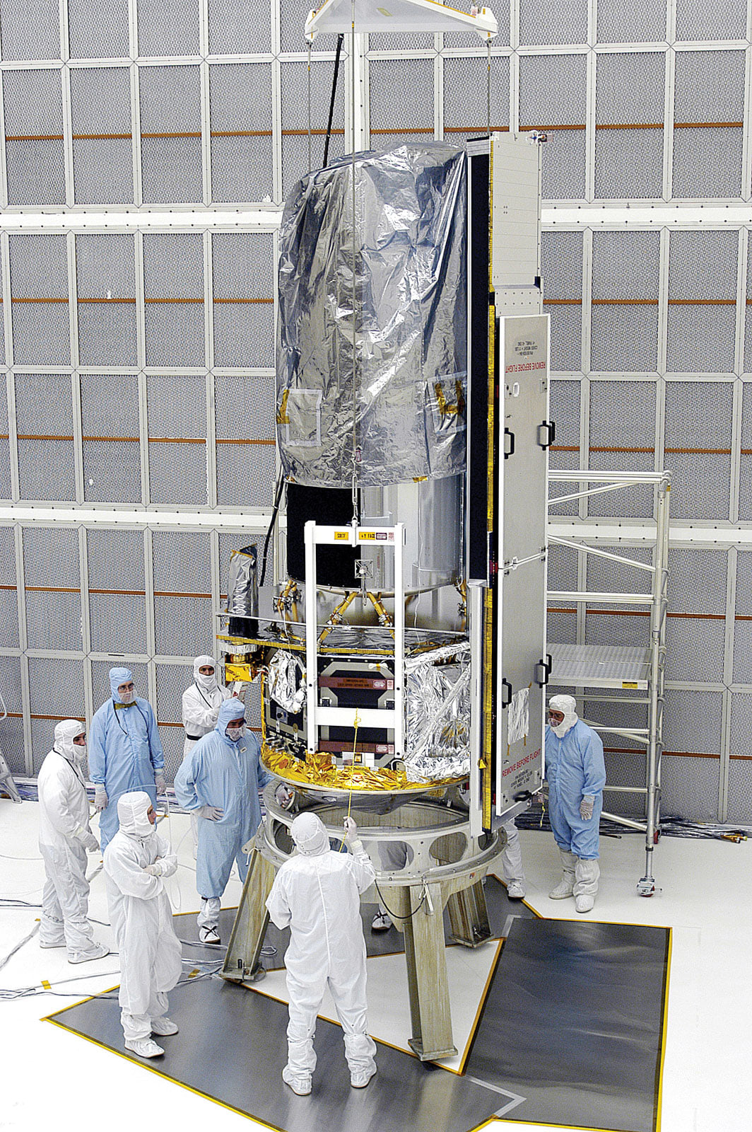
Figure 40.3 Eta Carinae nebula - showing dust being driven back by the stellar wind
Image Credit: NASA
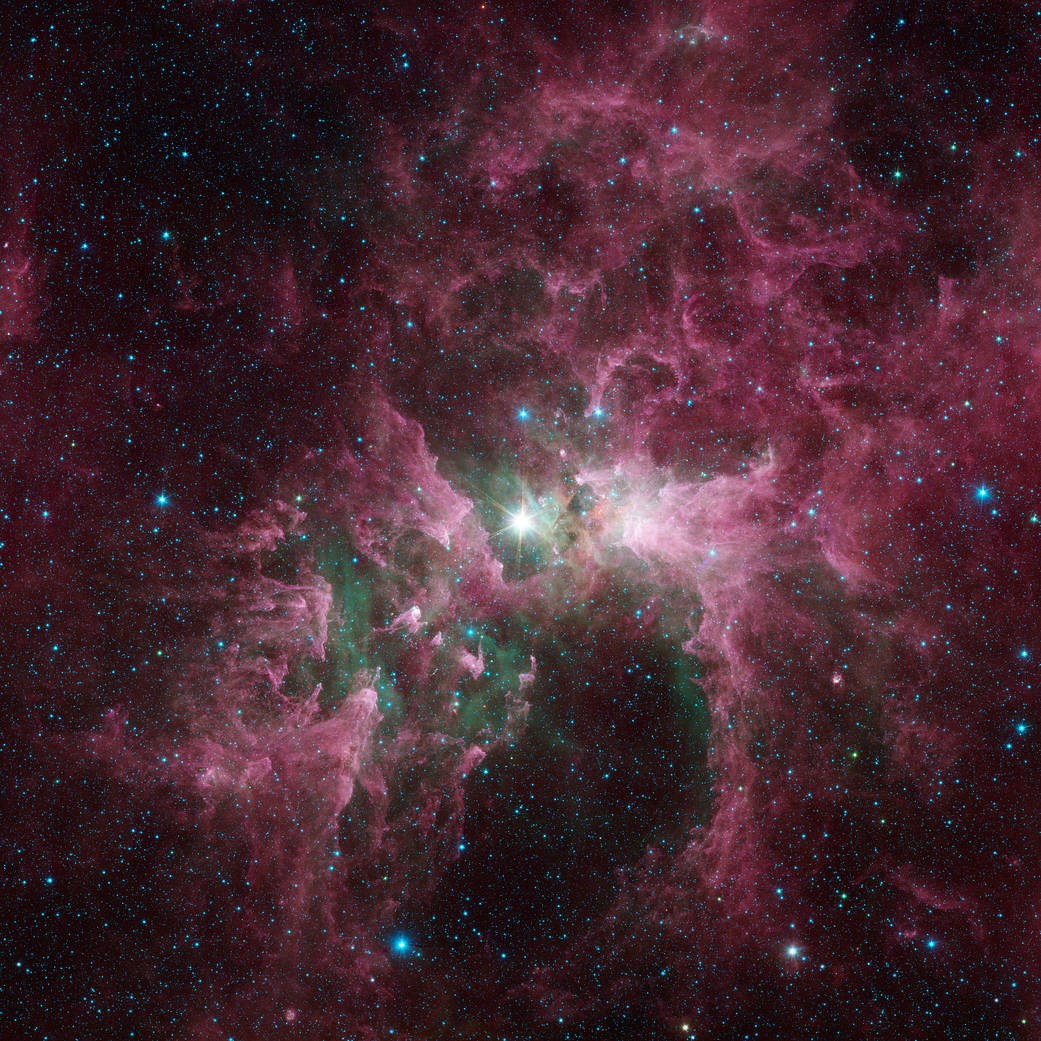
Figure 40.4 Planets of the Trappist-1 system compared with our Solar System
Image Credit: NASA
41: Gravity - LISA Pathfinder
If you know about gravitational waves, you probably know about LIGO, a pair of 4km-long interferometers, in different parts of the US, which have detected disturbances in the fabric of spacetime coming from neutron star collisions and merging black holes. The European Space Agency plans to go one better and deploy an observatory in space, using three spacecraft set up in a triangle 2.5 million kilometres to a side. The advantage of the location is that they don’t get all the vibration noise that LIGO has to filter out. But it was not certain that the technology could actually work. Was it possible for a laser interferometer to measure the position of a block of metal to the required accuracy? What effects would there be of solar heating, and interference from the spacecraft support systems?
To find out, ESA built and launched the LISA Pathfinder, a technology demonstrator for the first gravitational-wave detector in space. Instead of having three gold/platinum cubes 2.5 million km apart, it had two of these cubes, floating free about 40 cm apart. Because of the short ‘arm length’, it had no hope of measuring gravitational waves, but that wasn’t the point. The idea was to check that the laser system could measure the positions of the free-floating cubes to within the required 10 picometres (10-11 metres), and to measure possible interference from heat and magnetic fields.
LISA Pathfinder operated from 2015 to 2017, and was placed in an unusual ‘lissajou’ orbit in which it did loops around the Earth’s L1 Lagrange point - the point where the gravitational fields of the Sun and the Earth balance - a near perfect ‘free fall’ point. The mission was a success, the instruments were sensitive enough, and it provided the confidence required to allow ESA to go ahead with the full scale LISA. In the last few months of its operating life, LISA pathfinder contributed to the measurement of near-Earth asteroids - by picking up their minute gravitational fields as they passed.
Figure 41.1 Lisa Pathfinder
Image Credit: ESA

Figure 41.2 Schematic of the technology package showing the two gold/platinum cubes
Image Credit: ESA
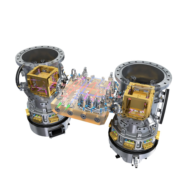
Figure 41.3 A valiant attempt to draw the trajectory & final orbit of LPF
Image Credit: ESA
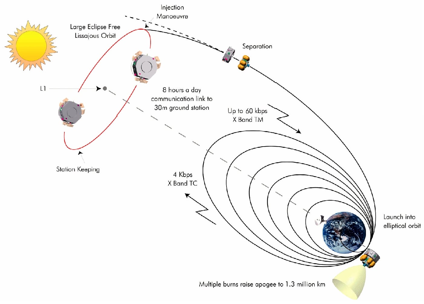
42: X-ray eyes - Chandra
At 22.8 tonnes, the 13m-high Chandra X-ray Observatory, including its solid fuel rockets, was the heaviest object ever carried by the Space Shuttle, when the Shuttle Columbia carried it up on 23 July 1999. Chandra orbits Earth in a very highly eccentric orbit ranging from more than 134,000 kilometres from Earth and then back to within 15,000 kilometres of Earth. X-rays are emitted by high energy processes, and are generally absorbed by the Earth’s atmosphere, so a space telescope allows us to see some of the most energetic processes & explosions in space. The data are particularly useful when combined with UV, optical and infrared observations from different telescopes looking at the same object.
X-rays can’t be focussed by a lens, so Chandra works by using a number of curved mirrors arranged in a kind of ‘funnel’, so that incoming x-rays glance off the surface and are channeled into a point, where the intensity is measured, and gratings are used to split the x-rays out by energy (by diffraction), so that the x-ray intensity and energy can be measured at the point the aperture is pointing at. This allows images to be formed using x-rays originating only from a specific chemical element.
Originally expected to last for five years, Chandra is still sending back data over 20 years later and has contributed to many scientific discoveries about stars, the planets of our Solar System, supernovae, black holes and neutron stars.
Figure 42.1 The 13m-high Chandra spacecraft
Image Credit: NASA

Figure 42.2 Supernova remnant in the LMC
Image Credit: NASA
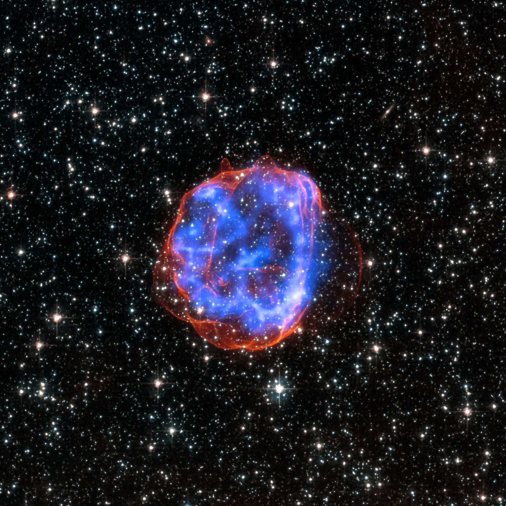
Figure 42.3 Bright x-ray flare from the supermassive black hole at the centre of the Milky Way
Image Credit: NASA
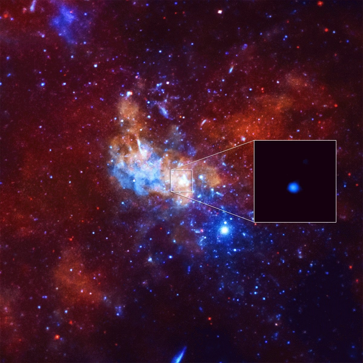
Figure 42.4 X-ray emissions from Jupiter
Image Credit: NASA
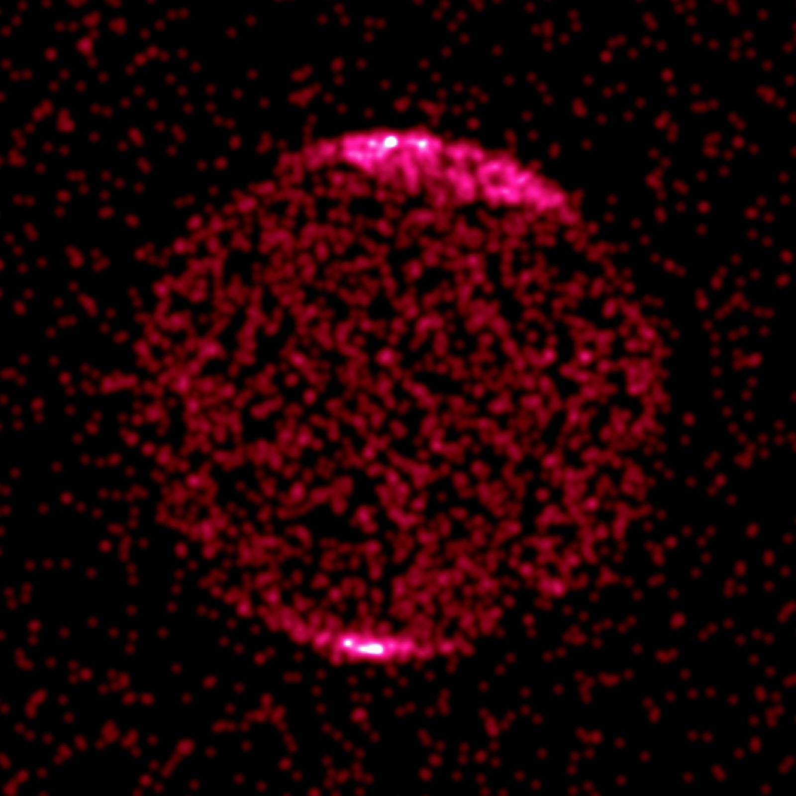
Figure 42.5 High energy x-ray-emitting jets spewed out by active galaxy, Centaurus A
Image Credit: NASA

43: Hubble!
The Hubble Space Telescope (an 11-tonne optical & infrared observatory) got off to a bad start after it was taken aloft in the Space Shuttle, Discovery, on 24 April 1990. The first images showed that something was badly wrong with the optical system. It was discovered that a 1.3mm misplacement in the optical measurement rig used to guide the grinding of the telescope’s 2.4m mirror had led to it being made with a conic constant of -1.014, when it should have been -1.002 - so the edges of the mirror were a whopping two-thousands of a millimetre out of place. Luckily, NASA was able to rescue the situation by hauling the telescope aboard a later flight of the Shuttle, and fitting a corrective lens at the front. From then on, amazing science and fantastic images were obtained.
The next major event in the history of the HST was in 2004, when NASA management said they would no longer maintain the spacecraft and it would be left to die. A wave of protest involving members of the public who had been rightly ‘wowed’ by HST’s astonishing images quickly led to political pressure and a backtrack by NASA. The 13m x 4m telescope continues to operate and, unless rescued, will begin to descend into the atmosphere sometime after 2028.
Astronomers are hoping that the next great eye in the sky, the James Webb Space Telescope, which is currently under construction, will be just as successful. I have just picked a few nice shots from Hubble but left out some of my favourites - like the ‘ultra deep field’. You can Google “Hubble top 100” to see more!
Figure 43.1 HST in flight, imaged from the Space Shuttle Columbia
Image Credit: NASA
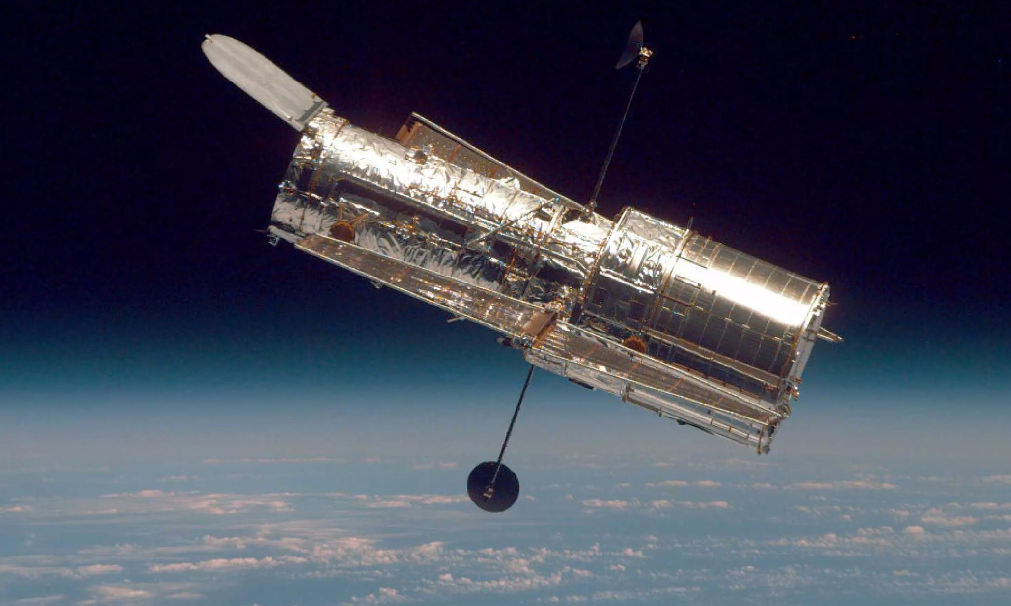
Figure 43.2 A shell of light, travelling at, well, the speed of light, illuminates dust which was emitted from the central star many millennia ago
Image Credit: NASA
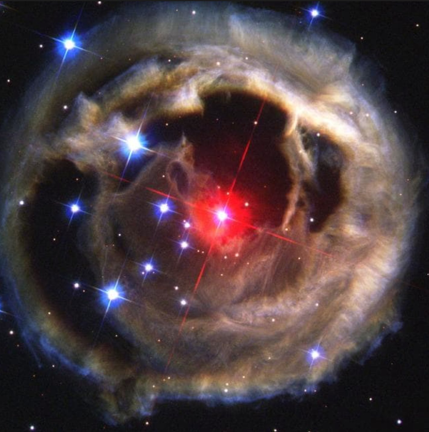
Figure 43.3 Three moon shadows on Jupiter
Image Credit: NASA
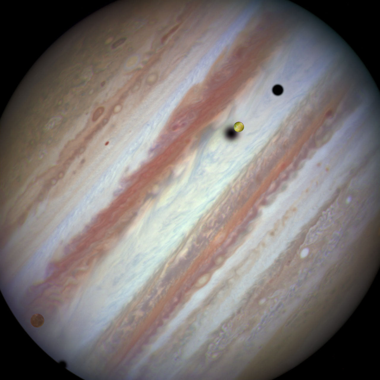
Figure 43.4 Dust cloud torn apart by stellar winds from newly ignited, hot, star
Image Credit: NASA
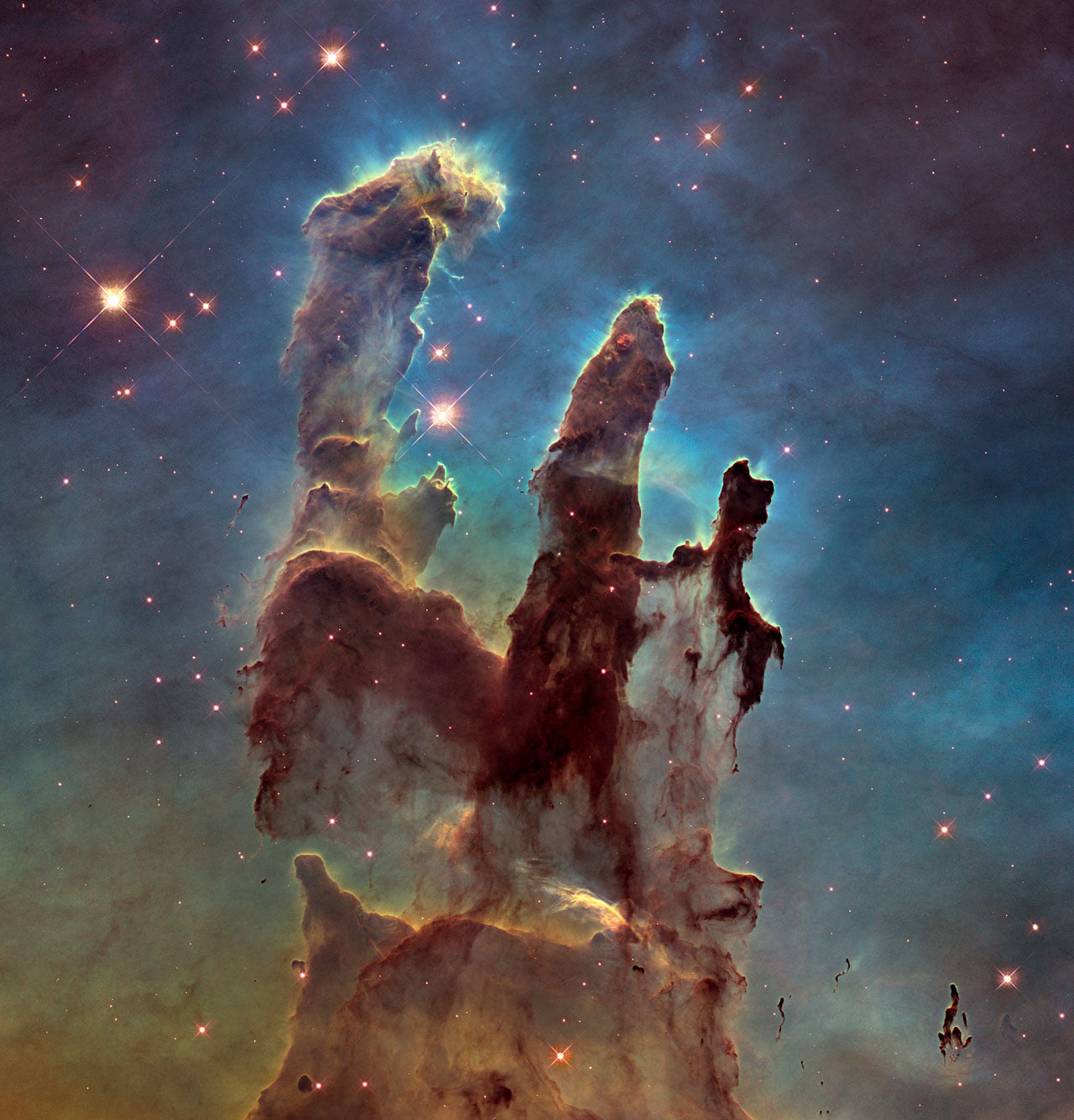
Figure 43.5 Stephan’s Quintet: Four red galaxies interact, while the blue one at top left is in a different neighbourhood.
Image Credit: NASA
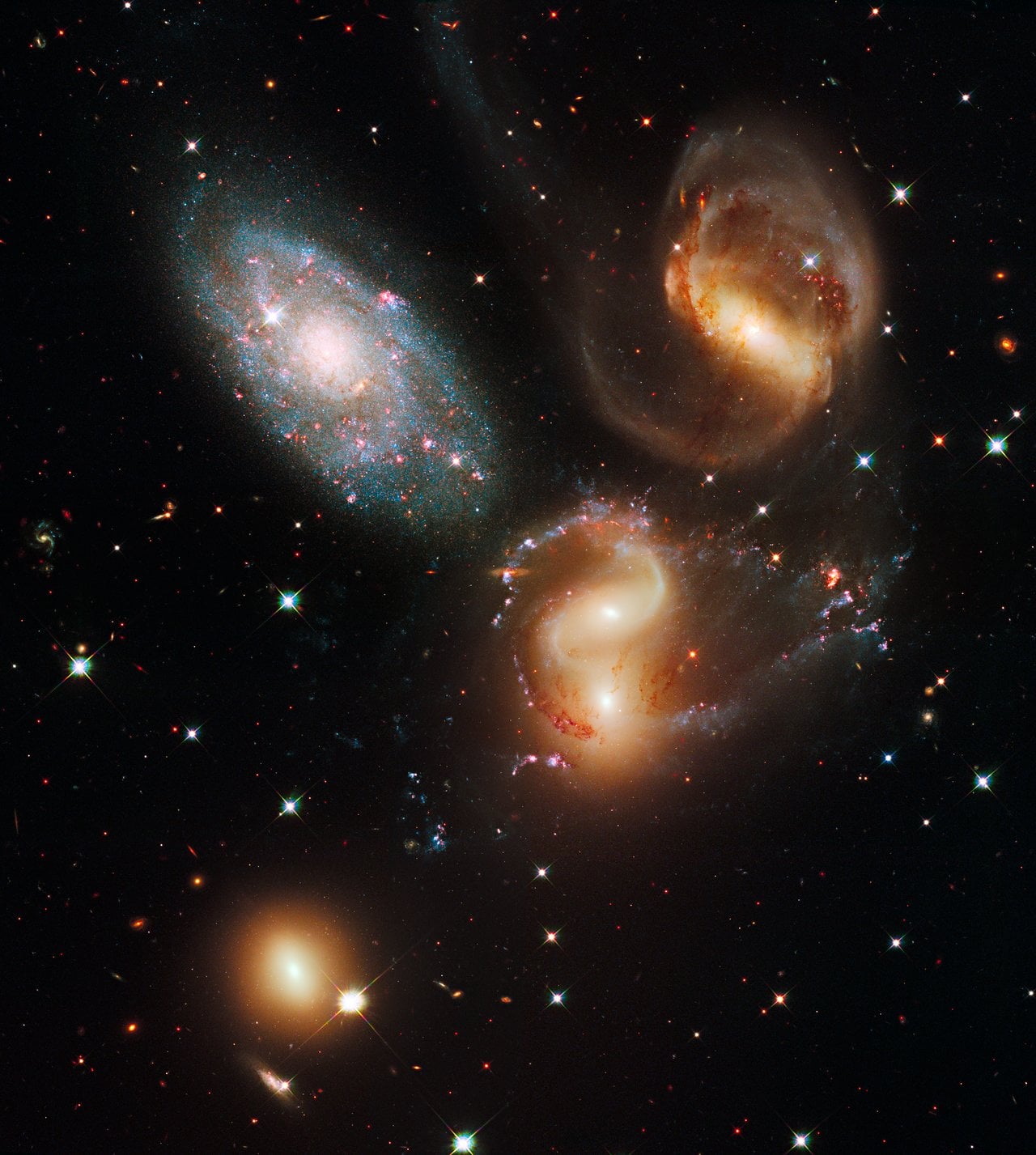
| Previous |
Author: Dr Ian Kemp (ICRAR), from content posted to the ASNSW Facebook Group, various dates in 2020. Last updated 18 July 2020.
